Wednesday, March 20, 2019

Raindrops keep fallin' (Erratum)

Raindrops keep fallin' (Erratum)
The error in the last post was that the rain rate was written as 1 drop/sec. whereas it should have been
1.0 drops/sec/cm2 (i.e. for a 10 mm x 10 mm starting grid).
Because of this I divided by the number of sites, quite arbitrarily. Numerically, the end result is the same, but the logic was wrong.
The plot of time T vs x is appropriately modified above.
At a completely uniform rate it would take 100 secs to cover 10 mm x 10 mm at this rate. corresponding to a rain rate of 36 mm/hr of 1 mm dia raindrops.
The times involved (in secs), corresponding to the above graph, are tabulated below:

size
total
99%
90%
50x50
840.15
458.55
230.08
40x40
795.53
457.46
229.98
20x20
656.99
448.67
229.14
10x10
518.74
418.74
225.71

The error is regretted!

Raindrops keep fallin'


Raindrops keep fallin’ on my head…

During the rainy season, sometimes one observes a gradual onset of rain. A drop falls at one spot on the ground, then at another nearby point, and so on. In one of Satyajit Ray’s films a raindrop falls on the head 
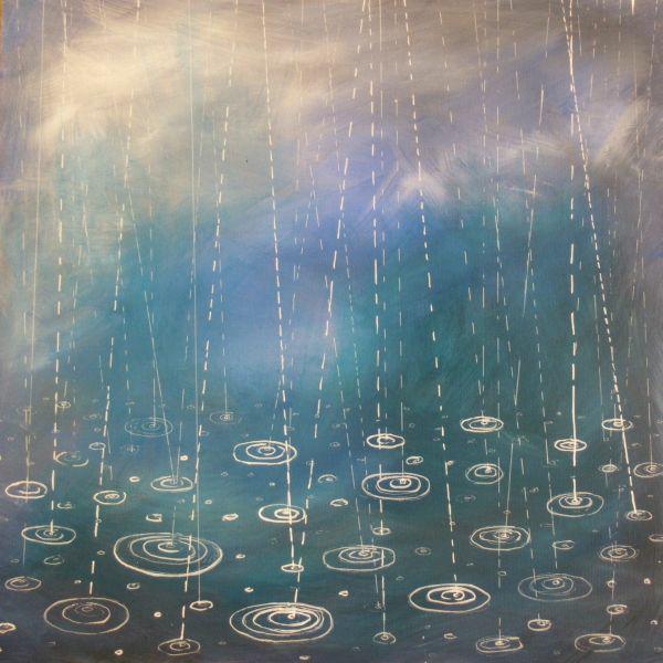
of a bald man (I can empathise with that!), and then many raindrops fall in the adjacent pond, each creating a set of ripples (as in Fig1 below).


Fig.1


Fig.2
So how long does it take before each point on the ground is covered by raindrops? So we can try to estimate this time, but making all sorts of assumptions. But… not for the case of the bald head, which would be problematic , since the drops will not stay in place!
Assuming 1 mm dia raindrops, you need 1 mm of rain on the ground to cover it (assuming raindrops as spherical – which is not the case). If the rainfall rate is 1 mm/hr it would need 60 mins!
The problem is an exact analog of getting one monolayer of atoms on a surface.
Assuming a 10 mm x 10 mm grid with 100 pixels (each of 1 mm x 1 mm size) and 1 mm dia raindrops, with 1 drop per sec, it would take a minimum of 100 secs.
If we take random falling of drops at the same rate, it takes more time (see below).
The difficulty with raindrops is that they are not of the same diameter (nor even spherical, due to the effect of drag). For atoms, assuming only one species of atoms and with the same isotope, there is no size variation.
a a)    assume all raindrops are the same size, 1 mm diameter  (unlike Fig.2 above) and the pixel size equals the diameter of the raindrop, assumed to be spherical.
b b) The rate at which raindrops fall is assumed to be constant (assumed as 1 drop/sec for convenience).
c c) The location at which the raindrop falls is assumed to be perfectly random.
d d) Implicitly it is assumed that the raindrops fall vertically (no wind) on a flat surface.
   e) The bouncing off and splintering of raindrops after hitting the ground is also neglected.
f  f) If more than one raindrop lands at the same site, there is no spillover (see below). This problem does not occur in molecular beam epitaxy, because one atom that lands on top of another will just bond with it (or get reflected off).

There is some scaling, obviously, here, both in time and in space. If we chose a rainfall rate of 0.2 drops/sec, the time required for each process goes up by 5X. Also, one could just as well have chosen raindrops of 2 mm diameter, and proportionately increased the total area to 20 x 20 mm2, without affecting the end result.

Thus, initially, no two raindrops are likely to land on the same mesh point. But, as coverage increases, it becomes increasingly unlikely that a fresh raindrop will find an unoccupied site. We assume no spillover: that is, even if multiple raindrops land at the same site, they do not spill over on to adjacent sites: this is clearly an unrealistic approximation, adopted for simplicity. (If the drop spills over, in which direction does it fall?).

The calculation of the total time taken to cover the surface assumes that each pixel will have at least one raindrop that has fallen on it. As coverage increases, the total time a raindrop has to hunt to find an unoccupied site increases proportionately to the fraction of unoccupied sites. A complete calculation would also show how the number distribution n(i,j), i.e. the number of raindrops that fell on each point (i,j), where the calculation stops when n ³ 1 for all i,j.Sticking to a 10x10 grid of pixels, the very first raindrop to strike takes just 1 sec to find its spot, while the very last raindrop has to make multiple attempts to find the very last unoccupied site, so it takes 100 secs to find it. Intermediate drops find their time in between these two limits, as calculated proportionately by:

Ti = 100/(101 – i), where i goes from 1 to 100.
And the total time is: T = STi, summing over all i.

It may be necessary to sum over a smaller number of sites: say i = 1 to 99 for 99% coverage (see below).
I did the summation in Excel, but it could be implemented in other ways as well.

The next question that occurs is: what happens if we increase the grid size from 10x10 to 20x20, keeping all else the same? The above formula gets appropriately modified, which is straightforward. But the total time to cover the surface increases. This is what one would expect. So, something should converge – but what? The total time per site may converge (divide the total coverage time by the total number of sites). This is plotted in the Figure 3 below, as the topmost curve. If the curve is converging, it’s going to take a while! But a little reflection will show that it will never completely flatten: as you keep increasing the grid area, there will be some pixel somewhere that will not get covered – but clumps and blobs will get more and more drops. 
Fig.3
With a 10x10 grid, the if we leave out the last raindrop, that corresponds to 99% coverage. For a 50x50 grid, missing the last drop works out as 99.96% coverage.

So actually, it makes more sense to look at 99% and 90% coverage, which is what is shown in the two lower curves of the graph. And these do saturate. 
For a 10x10 grid, and 90% coverage it takes 226 secs (instead of 100 secs if everything was uniform), and for 99% coverage, 419 secs. For a 50x50 grid (a better approximation), it takes 230 secs for 90% coverage, and 459 sec for 99% coverage.

But one thing is clear: there is no one answer to the question,” How long does it take for rain to cover the surface?” – unless you specify the coverage.

As mentioned above, this problem is analogous to the case of molecular beam epitaxy (MBE), which also has a layer-by-layer growth mode. MBE also has two other growth modes, but those are applicable only for atoms that can bond to make solid layers. Another difference from MBE is that rainfall takes place from fairly large clouds, whereas in MBE the effusion cells are quite small, and close to the substrate, so geometry effects dictate a cosine dependence on angle.

Of course, the above analysis has made a number of assumptions, listed above. The requirement of perfect randomness may not be met. The assumption that all raindrops fall vertically is also unrealistic: a slight, localized breeze will make nonsense of that.
Finally, the method of calculation used above may not be rigorous: it will apply only on average.
The right and proper way is to do Monte Carlo – which I have no intention of doing. I’m sticking to my own pay grade.


Friday, March 8, 2019

Closing the door


The problem of opening and shutting doors plagues the refrigeration and air conditioning businesses. How many times per hour can one allow those pesky customers open a door to an AC area without adding to the heat load too much? Or those people who complain the refrigerator is not cooling effectively, when they keep opening the fridge door wide? But the problem that bothers me is: how much air pollution (PM2.5) is getting in to my living room each time the door is opened to the balcony whose air is not purified? In my friend Chandan’s living room the PM2.5 level immediately responds, going up by easily 10-20%.
A strip of the door of height h and width dx has an area dA (Fig.a):
                                                                
                                                              dA= h dx                                                                                                                                                                         
When the door is being shut it has an angular velocity w and if r is the distance from the pivot point, the velocity v at that point is given by (Fig.b):   
                                               
                                                            v = wr

where r can be calculated from the distance x and the perpendicular distance y (see part b) of above diagram):

r = (x2 + y2)1/2

Let  nbe the number of particles of PM2.5 in the room initially. Then the rate of change of n is given by:

dn/dt = nov dA

But the velocity v is independent of time, and so it is also independent of y. Setting y = 0, r = x:
dn/dt = now òh x dx = now h d2/2

So that, since door area A = hd and taking Dq = wDt:

Dn = A (Dq) d n0

where x is integrated across the width d of the door, and x  = 0 at the pivot of the door. Of course, this assumes that the time period when the door is being accelerated to velocity v, and when it is decelerated to zero velocity, is negligible. Also, the temperature is being assumed to be the same in both rooms 1 & 2, as is the density. This may not be a very realistic assumption and, indeed, others do not make it (see below).
Take n0 = 3x1025 m-3 (1 atm at normal temperature & pressure), h = 2 m. d = 1 m, and    Dq = w(Dt) = p/4 (45° door opening). 

so that  Dn is independent of the time taken, and only dependent on the angle Dq traversed.
So: Dn = 2.36 x 1025 atoms
A room of volume 22.4 m3 contains 6x1026 atoms (1000 mols x Avogadro number, at NTP), so the Dn = 2.36 x 1025 atoms corresponds to 0.88 m3. That is, opening the door by this much allows about 4% of the outside PM2.5 contamination to get in: so the PM2.5 level increases by about 4% of the outside PM2.5 level (for every 45° opening). For a 90° opening, it should be ~8%.

As a reality check: if we assume a 45° angle (which is what we did), the volume pushed out by the door while closing is (pr2/8)(h) = 0.78 m3.

The latter volume is 88% of the former, so a 12% difference can be attributed to the fact that the velocity v is not constant across the door (in the x-direction).

The amount of 880 L is probably an overestimate because the angular velocity w is assumed to be constant while the door is moving, whereas it is more likely that it starts from zero and increases.

But if it is only dependent on the angle Dq traversed then the time variation of the angular velocity will not matter.

This analysis will work if the door is closing: moving CW about its hinge so that air is being forced from Room2 to Room1.

However, if it is opening (moving CCW), the air from room 1 is not being pushed, but pulled (while the air already in room 2 is being pushed CCW).

The analysis for that case is different: so opening and closing the door gives rise to different effects - and I shall not go there.

I found 4 papers in the literature that tackled a similar topic albeit with different assumptions.

Foster et al [1] refers to the case of an air curtain above the door so it is not directly applicable, and it has an analytical solutions as well as a computational fluid dynamics (3D CFD) study.

Lagus [2] considers a pressure difference between both rooms with buoyancy effects driven by the difference in densities in the two rooms. But, for the case of equal density, no buoyancy effects occur, and the volume displaced by the door is given by:

Vp = A(Dq)d/2
which is similar to that derived above for Dn.

Hendiger et al [3] also consider the flow rate due to a pressure difference between the two rooms, and obtain the flow rate Q as:

Q  (m3/s) = 0.067 (Dp)0.63

Where Dp is in Pa, and the exponent n is usually between 0.6 and 0.7. They also conclude that: “quick door swing causes a greater transfer of contaminants, regardless of the width of the door opening, which shows that it is necessary to open the door more slowly.” [3].

Marshall et al [4] have derived an expression – using very similar logic to that gven above – but specifically trying to calculate the force required to close a door, overcoming air resistance. They show that the force required is pretty low, until the point where it is almost shut, and there it increases sharply for the last few degrees of shutting it:
“When the windows in a small room are shut, the effect of displacing air as the door is pushed makes the door more diffcult to push when it is nearly closed.”
 But they add that air flow under the door will reduce this effect somewhat at small angles.

A more complete analysis would take into account temperature and pressure profiles (as has been done [1,2,3] by other authors. But simply the effect of door swing has also been considered [2.4], although the latter is more rigorous since it takes acceleration into account.

1 1)    “Three-dimensional effects of an air curtain used to restrict cold room infiltration” A.M. Foster et al Applied Mathematical Modelling 31 (2007) 1109–1123
2 2)     “Air inleakage due to door opening and closing” P.L.Lagus (26th Nuclear Air Cleaning & Treatment Conference, Sep.2000)
3 3)     “Influence of the Pressure Difference and Door Swing on Heavy Contaminants Migration between Rooms” Jacek Hendiger  et al PloS One 11(5): e0155159. doi:10.1371/journal.pone.0155159 (11th May 2016)
4 4)     “Slamming doors due to open windows”, D.A.Marshall et al J.Phys. Special Topics A2.7 (23Nov.2011)