Heterogeneity Lowers Herd Immunity, but Overshoot is still there

In a recent article, Apoorva Mandavalli [1] asks if we are closer to herd immunity than previously believed.  She discussed three papers that discuss lower herd immunity thresholds (HIT) due to heterogeneity in the population. All three papers use SEIR models, but with varying approaches. The papers by Lourenco et al [2] and by Gomes et al [3] are less easy to use, but the paper by Britton et al [4] is more understandable. Mandavalli [1] also discussed these papers with other scientists to get an idea of whether a new scientific consensus is emerging.

The reason why this question is pressing is that we all want to know: when will it be over? Conventional HIT values are given in the 60-70% range. These authors argue that it could be lower. Indeed Britton’s value of 43% (higher than the other two) may have informed the Swedish ‘hands off’ attitude of ‘voluntary compliance’ in the last few months, along with the attitude that everybody is going to get infected sooner or later, no matter what we do. In this post, as before, I want to calculate the cutoff percentage X_co at which the epidemic actually stops [5], which is higher than the HIT, which is merely the point at which the number of infectious cases peaks, and herd immunity effects start to kick in. These papers have been widely discussed by several authors [6- 14], and various points that they have raised will be discussed later.

Lourenco et al [2] state that the standard formula for the herd immunity threshold (HIT):

HIT = 1 – (1/R₀)

is modified if a fraction r of the population is resistant to infection, becoming:

HIT = (1 - r){ 1 – (1/R₀)f} where:

f = 1/[1 – (c₁/c₂){r/(1 - r)}(1 - d)]

where c₁ and c₂ are the contact rates for the two sub-population groups, and the interaction matrix (of the two sub-populations) d. The parameter d lies between 0 and 1.

This equation for HIT suggests that a wide variation in HIT will occur depending upon: (i) the proportion that is resistant to infection (ii) the R0 within the non-resistant group, and (iii) the degree of mixing between the two groups.

a)      When d = 1, there is no mixing between the two sub-populations, it is assortative within the groups;

b)      Random (or proportionate) mixing occurs when d = r; HIT reduces to the expression:

HIT = 1 – (1/R₀)  – r.

c)       when d = 0, there is maximal mixing between the two subgroups.

 

What is not clear is: what is the difference between (b) and (c), between random and maximal mixing?

The proportion r of the sub-population 1 being resistant to infection means R_0,1 = 0. The group specific R_0,I  = b_i c_i/s_I is the R₀ of the i^th group, or the fundamental transmission potential of the virus within a homogeneous population consisting of members of that group. The rates of loss of infection and immunity are given by respectively by s and g.

a)      In the no-mixing (fully assortative) case (when d = 1), f =1, and the herd immunity threshold reduces to: HIT = (1 - r) (1 – 1/R₀). That is,   for this case, HIT declines in proportion to the size of the resistant group.

However, this is not very clear: if there is no mixing between groups 1 and 2, why should HIT for group 2 be independent of r, and given by the standard expression for HIT? Especially since the standard HIT does not involve the size of the population?

 

b)      But for random mixing (c₁ = c₂ Þ d = r):  z* = 1 – (1/R₀) - r. That is, the virus will not spread if r ³ 1 – (1/R₀). This is the standard case, because there is no difference between sub-groups 1 and 2 (z is the sum of the numbers of infected and recovered persons).

 

If c₁ ¹ c₂, random mixing occurs when d = r c₁/[r c₁ + (1 - r c₂)]

 

c)       Maximal mixing case (d = 0): the authors do not pursue this case. Also, it is not clear: what is the difference between random mixing and maximum mixing?

 

The authors conclude:

“The drop in HIT is proportional to the fraction of the population resistant only when that fraction is effectively segregated from the general population; however, when mixing is random, the drop in HIT is more precipitous.”

 

In addition, they also add that their results are similar to those of Gomes et al [3] but that their values are lower than those obtained by Britton [4].

I have a couple of doubts about the paper by Lourenco…Gupta [2] which I have mentioned above. However, since I have not derived the equation used by that group, it may not be fair to comment.

Gomes [3] argues that “individual variation in susceptibility or exposure (connectivity)

accelerates the acquisition of immunity in populations due to selection by the force of infection.”

The paper of Gomes et al [3], using a SEIR model, assumes variable susceptibility and exposure, and both susceptibility and exposure (connectivity) are given by gamma distributions. The gamma distribution is fitted to experimental data for 11 countries, but one fitting parameter is the coefficient of variation, CV, defined as the ratio of the standard deviation to the mean. (The infectiousness of exposed individuals is assumed as half of that of exposed individuals; the incubation period is 4 days and the period of infectiousness is assumed as 4 days).  Gomes et al use values of CV ranging from 0 to 3, and plots the herd immunity threshold HIT vs variable CV. For CV = 3, they get values as low as 10%. We will return to Gomes later. The results of Gomes will be discussed later.

Let’s now look at Britton et al [4].

 

Traditionally:

Table 1:

 

R0	h0 = 1 - (1/R0)	xco
2	0.5	0.8
2.5	0.6	0.89
3	0.667	0.94

 

H₀ is the herd immunity threshold, x_co is the population cutoff fraction at which infection stops (Bastin [5])

R₀ = - [ln(1-x)]/x

Britton takes into account age structure & variable social activity to obtain a value h_aa. Specifically, the population is divided into 6 different age groups (0-5, 6-12, 13-19,20-39, 40-59 and 60+ years) and three different activity levels (normal, doubled and half).

Table 2:

R0	haa = 1 - (1/Re)	Re
2	0.346	1.53
2.5	0.43	1.75
3	0.491	1.96

 

The equation h_aa = 1 - (1/R_e) is an assumption to create an effective R-number R_e for the situation of age structure & variable social activity. It may not be valid (but it turns out OK!).

Fitting the data of R_e vs R₀ yields a linear plot:

R_e = 0.672 + 0.43R₀

We can use this to extrapolate to values of R₀ other than those calculated by Britton.

R_e = ln(s_¥)/[ 1 – s_¥]

Varying R₀ one can generate a plot of s_¥ vs R₀ accounting for age structure & variable transmissibility:

Table 3:

R0	haa = 1 - (1/Re)	Re	Xco
1.5	0.241	1.32	0.43
2	0.346	1.53	0.60
2.5	0.43	1.75	0.71
3	0.491	1.96	0.78
3.5	0.541	2.18	0.84
4	0.582	2.39	0.88

 

We are also assuming that the equation above for calculating the population cutoff X_co remains valid when we plug into it the effective R-value, R_e.

The extrapolation of R_e vs R₀ to values other than those calculated by Britton (R₀ = 2, 2.5 &3) is relatively more reasonable, since the plot seems to be linear. But it is an assumption, to be sure.

 

X_co takes into account overshoot along with age and variable activity. This is the fraction at which the epidemic stops.

Fig.1: age & activity [4]

The lower curve is the herd immunity threshold as calculated by Britton, for the case of age structure and activity structure. The upper curve is the population fraction at which the epidemic dies out completely and no more infections occur.

Britton has two more columns, in which he accounts for only age structure and only for variable activity. Using similar logic for the social activity – which Britton says is more important:

R_e = 0.603 + 0.50R₀

Table 4:

 

R0	haa = 1 - (1/Re)	Re	Xco
1.5	0.261	1.35	0.46
2	0.376	1.60	0.64
2.5	0.460	1.85	0.75
3	0.524	2.10	0.82
3.5	0.575	2.35	0.87
4	0.616	2.60	0.90

This plot looks almost the same as the previous one – but it is displaced slightly upwards.

 

For the case of age-structure only:

R_e = 0.21 + 0.82R₀

Table 5:

 

R0	haa = 1 - (1/Re)	Re	Xco
1.5	0.305	1.44	0.54
2	0.459	1.85	0.75
2.5	0.558	2.26	0.85
3	0.625	2.67	1.00
3.5	0.675	3.08	1.00
4	0.713	3.49	1.00

 

 

 

Fig.3: age structure only [4]

 

This plot, for age structure only, is clearly pushed upwards – especially for R₀ of 3 and above – where it hits 100% of the population.

Of course, as R₀ increases, the percentage asymptotically increases towards 100% and does not actually reach a hundred – the above results are due to numerical inaccuracies.

Britton says that the activity structure is dominant and the age structure does not play so much of a role (roughly activity is 3X as important as age in his calculations).

The data given by Lourenco et al [2] can be handled similarly. However, the values of HIT – as pointed out earlier – are much lower:

This table (1^st 2 columns from Table 1 in Ref.2) is for assortative mixing (i.e. no mixing of groups 1 & 2):

Table 6:

 

R0	heff = 1 - (1/Re)	Re	Xco
1.5	0.16	1.19	0.30
2	0.25	1.33	0.45
2.5	0.30	1.43	0.53
3	0.33	1.49	0.57

 

Similarly, for proportionate mixing:

Table 7:

 

R0	heff = 1 - (1/Re)	Re	Xco
1.5	0	1	0
2	0	1	0
2.5	0.10	1.11	0.19
3	0.16	1.19	0.30

 

Fig.4: assortative and proportionate mixing [2]

The values for h_eff and X_co are shown in Fig.4 for both assortative and proportionate mixing.

 

Gomes et al [2] considered variable susceptibility and variable connectivity (separately) – but also mentioned the ‘final size of the uncontrolled epidemic’ in their Fig.3. This is listed in the 3^rd column 9in the two Tables below) and compares pretty well with the value of X_co (in the 5^th column in the two Tables below) as calculated from R_e (obtained as above from h).

Gomes et al [2] has only considered R₀ = 3 but with variable susceptibility CV (as mentioned above):

Table 8:

 

CV	heff = 1 - (1/Re) (from Gomes)	Final % of epidemic (from Gomes)	Re	Xco
0	0.65	0.94	2.86	0.93
1	0.43	0.67	1.75	0.71
2	0.2	0.33	1.25	0.37
3	0.1	0.17	1.11	0.19
4	0.07	0.11	1.08	0.14

 

This is shown graphically:

Fig.5: variable susceptibility [3]

 

Gomes et al [3] has only considered R₀ = 3 but with variable connectivity CV (as mentioned above):

Table 9:

 

CV	heff = 1 - (1/Re) (from Gomes)	Final % of epidemic (from Gomes)	Re	Xco
0	0.65	0.94	2.86	0.93
1	0.31	0.54	1.45	0.55
2	0.12	0.23	1.14	0.23
3	0.07	0.125	1.07	0.12
4	0.04	0.08	1.04	0.07

 

In this case, the values of X_f and X_co agree somewhat better:

Fig.6: variable connectivity [3]

Neither Lourenco [2] nor Britton [4] mentions overshoot, but Gomes [3] clearly does by tabulating X_f (the final composition of the population after the epidemic is over)

Making some assumptions, we have calculated the value X_co at which transmission of the virus completely stops. These assumptions may not be correct – but the conclusions are plausible. And they do match pretty well with the calculations of Gomes [3] – although the matching is better for the variable connectivity case (Fig.5) than it is for the variable susceptibility case (Fig.4).

Discussions:

At this point, it is worth examining what various authors [6-14] have concluded, based on the three papers and their understanding. Since there is considerable overlap, only some points will be taken up.

Jha [6] discusses Sweden’s approach of voluntary compliance and the statistics that show that Sweden did better than the UK – but significantly worse than its Nordic neighbours, and attributes the high death rates to a flawed approach to taking care of the elderly in care homes and foreign migrant labour in crowded urban areas. He points out that 85% of Sweden’s population lives in cities and that the elderly in Sweden’s care homes were already frail (28% of men and 19% of women would die within 6 months of entering the facility, in normal times) and where half of all deaths occurred. Anders Tegnell expected 25% of the population to contract the virus based on Britton’s model [4], while in crowded Stockholm it was a little more than 20%. However, Johann Giesecke still argues that, despite setbacks, the Swedish strategy as a whole is not disqualified. Indeed, he said,” I expect when we count the number of deaths in each country in one year from now, the figures will be similar, regardless of the measures taken.” Giesecke has heavily criticized Ferguson’s paper as fundamentally flawed by debatable assumptions, which nevertheless, provoked ‘a huge over-reaction’ all over the world, but especially in the U.K. and the U.S. Needless to say, Giesecke does not mention the cutoff X_co and sticks to the HIT.

Vineeta Bal [7] discusses the results of serological surveys in India: particularly Delhi (23% sero-positivity), Mumbai (40%), Berhampur (31%). She also points out that it was 51.5% in Pune, ranging from 65% in the most crowded districts to 31% in the least crowded districts. Similar results were obtained in Mumbai (16-57%), with the highest sero-positivity (57%) in the slums of Dharavi. However, Vineeta Bal emphasizes that these tests do not mean that the residents of Dharavi are immune, because the serological test used only detects antibodies, not ‘neutralizing antibodies’, which confer immunity (and are more difficult to detect. It will take 6 weeks to get results, according to Arunab Ghose of IISER). So, while the number of cases in Dharavi has come down, it is premature to conclude that it is because of herd immunity.

The town of Bergamo, the epicenter of the covid-19 outbreak in Italy, recorded 57% of the population had developed antibodies [8].

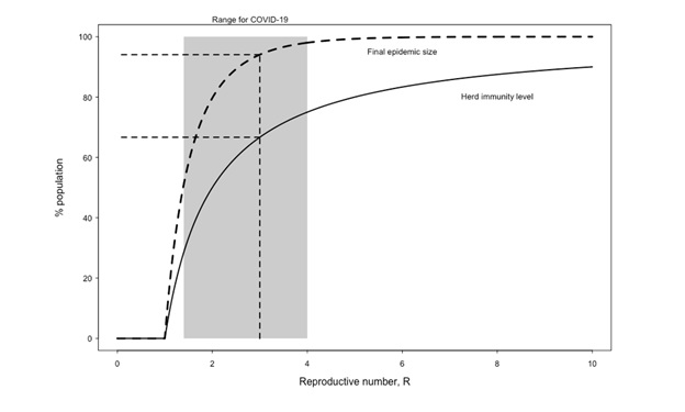
Fig.7: HIT & X_co vs R₀ from [9]

The above figure is from Kleczkowski [9], and it plots both HIT and X_co as a function of R₀. Kleczowski is rather balanced, merely pointing out that the concept of herd immunity is ‘not without controversy’ and would lead to a large number of excess deaths. Kleczkowski accepts that diversity (heterogeneity) in the population will lower the HIT from the 60-70% value for a homogeneous population to  a value as low as 10%, and mentions the above 3 papers.

Hartnett [10] also points out that in some cases the threshold could even be higher, e.g. in a nursing or care home. But, ‘on a larger scale’ any heterogeneity in the population (a variable R0) will lower the threshold, since the virus will first pick off the more susceptible but the epidemic slows down when it starts coming up against  less susceptible hosts. Tom Britton feels now that 43% is too high, and that additional sources of heterogeneity, not considered in their published model, may lower the threshold even more. Gabriela Gomes believes that Madrid may be approaching the 20% threshold that their group has calculated. Many other experts, according to Hartnett, believe that these studies are not completely reliable and are cautious about endorsing them, because behavior of people is often random and difficult to model. Kate Langwig (a co-author of Gabriela Gomes) feels that estimating heterogeneity is indeed difficult but it is important to do it: “We have been sloppy in thinking about herd immunity”. Jeffrey Shaman of Columbia objects that 20% is not consistent with other respiratory viruses: if it isn’t 20% for flu, why should it be for covid-19?

Hamblin [11] has discussed Gomes’s paper and introduces chaos into it, arguing that Gomes works on chaos, even though she does not use the word anywhere in her paper. Nevertheless, Hamblin says that dynamic systems can be unpredictable and small changes in susceptibility can lead to large consequences for the outcome of the epidemic - which may be a factor in the low predictability of pandemics. Britton does not think 20% is likely, and favours a higher number. Marc Lipsitch (of Harvard and author of ‘Rules of Contagion’) initially quoted 40-70% but, in later discussions with Hamblin, lowered his estimate to 20-60%, but with an increasing degree of skepticism as the threshold approaches 20%. Shweta Bansal also argues that under certain conditions (nursing homes) the threshold could exceed 70%.

Harry Stevens [12] quotes Yale epidemiologist Marcus Russi to say (about the U.S.) that: “There’s just way too little seroprevalence in all of these states to come anywhere close to achieving herd immunity.” But the higher range of sero-prevalence estimates in the U.S. is 25% - which is much lower than traditional values – but in the same ball-park as the estimates of Gupta [2] and Gomes [3] – but lower than that of Britton [4]. Stevens [12] does not mention the three papers being discussed here.

Fig.8: Herd immunity threshold and Overshoot [13]

Bergstrom and Dean [13] wrote in the NYT about ‘overshoot’ beyond the HIT, and emphasize that when we reach the HIT: “That’s not when things stop — it’s only when they start to slow down.” They also do not discuss the three papers, sticking to the original values of ‘nearly two-thirds’ of the population. According to Bergstrom and Dean:  “A runaway train doesn’t stop the instant the track begins to slope uphill, and a rapidly spreading virus doesn’t stop right when herd immunity is attained.”

Regalado [14] quotes a tweet by Florian Klemmer: “It seems there is the ‘herd immunity is already reached’ team and the ‘we are all going to die’ team. The good thing is, there is a third, ‘let’s get the data and let’s look at what this all means’ team out there.” Regalado also quotes Marc Lipsitch to say that the disease itself, when it causes herd immunity, does so more ‘efficiently’ than giving out the vaccine at random. According to Youyang Gu, roughly 10% of the U.S. population has now been infected. But, estimates vary widely: 10-80% of the population might have to be infected, depending on how well the virus spreads, but also on social factors like how much people ordinarily mix with one another (to achieve herd immunity).

Apoorva Mandavalli [1] points out that in some clinics in the U.S. as many as 80% of people who were tested had antibodies to the virus, with teenage boys having the highest prevalence. In Queens the prevalence was as high as 68%, while it was as low as 13% in Brooklyn. Most experts that Mandavalli discussed the papers with were not willing to accept herd immunity thresholds as low as 10-20%. Biostatistician Natalie Dean asked: where is the evidence that the detected antibodies are actually immuno-protective? Carl Bergstrom argued that, while such low herd immunity thresholds, were mathematically possible, these models are, at the moment, ‘guesses’. Other experts pointed out that all models are flawed because they over-simplify reality and do not accurately represent real world conditions. Jeffrey Shaman considered Gomes’s model as a ‘possible solution’ but questioned the wide range of parameters for different countries in the study. Most researchers are wary of concluding that the hardest-hit neighborhoods of Brooklyn, or even the blighted areas of Mumbai, have reached herd immunity or will be spared future outbreaks.

Franks and Roclov [15] point out that the percentage of antibodies observed in the Diamond Princess was about 20%, and similar numbers have been obtained in Stockholm, New York and London – suggesting that there is something in the 20% idea. However, the prevalence was as high as 54% in the Hartsville Correction Center. The authors discuss the idea of ‘immunological dark matter’, first mentioned by Friston [16] (50% of any population is not susceptible to infection because of cross-immunity from other infections and geographic isolation), but point out that the fact that values much higher than 20% mean that the T-cell innate immunity hypothesis remains to be proved. Finally, if a 20% threshold does exist, it applies to only some communities, depending on interactions between many genetic, immunological, behavioral and environmental factors, as well as the prevalence of pre-existing diseases.

Resnick [17] discusses the possibility that immunity may have a limited shelf life, maybe as little as 3 months. Under such conditions, the ‘let it rip’ approach to going for herd immunity in a society by uncontrolled (or lightly controlled) infection, may not make much sense. Resnick also discusses the various tests for viruses, antibodies, T-cells, B-cells etc. Resnick [18] also quotes Harvard epidemiologist Stephen Kissler [19] who advocates ‘stop-and-go’ social distancing and predicts that it might take till 2022 to build up enough immunity in the population, if it is done in a cautious manner.

Overall, the consensus seems to be that heterogeneity does lower the herd immunity threshold, but whether it goes as far down as 10% is not clear. Britton’s paper is the only one to be peer-reviewed, and in the paper the authors state that the calculated values are ‘indicative’, not set in stone. The point I want to emphasize in this post is that even if heterogeneity reduces the herd immunity threshold to values as low as 10-20% - which most experts believe to be unlikely – the fact of overshoot cannot be ignored. Sunetra Gupta [2] is well aware of overshoot, but only Gabriela Gomes [3] actually gives the values in her paper (as given above in Tables 8 & 9). The cutoff values X_co are significantly higher. It is these values that should concern us – when the epidemic is over, not when it peaks. The values quoted above for serological studies in London, New York, Stockholm, Mumbai etc refer to points in time where the epidemic is definitely past its peak, if not exactly ended, so the appropriate number is the cutoff X_co, not the herd immunity threshold. 

 

References:

1.       Apoorva Mandavalli https://www.nytimes.com/2020/08/17/health/coronavirus-herd-immunity.html

2.       2. Jose Lourenco… Sunetra Gupta  medRxiv 16^th July 2020 https://doi.org/10.1101/2020.07.15.20154294

3.       M.G.M.Gomes et al  medRxiv 2^nd May 2020

 https://doi.org/10.1101/2020.04.27.20081893

4.       Tom Britton et al Science 14^th July 2020  Science 10.1126/science.abc6810 (2020).  

5.      5. G.Bastin: “Lectures on mathematical modeling of biological systems,” 22^nd Aug.2018 (GBIO 2060)

6.       6. Ramanath Jha, “Sweden’s ‘Soft’ COVID-19 Strategy: An Appraisal,” ORF Occasional Paper No. 258, July 2020, Observer Research Foundation

 

7.       Vineeta Bal and Satyajeet Rath https://indianexpress.com/article/explained/sero-surveys-during-covid-19-why-do-they-matter-what-do-they-say-6558977/

 

 

8.       Niclas Rolander https://theprint.in/world/sweden-proves-surprisingly-slow-in-achieving-herd-immunity/443329/

 

9.       Adam Kleczkowski https://scroll.in/article/968357/why-herd-immunity-may-not-be-the-perfect-solution-to-coronavirus

 

     10 Kevin Hartnett https://www.quantamagazine.org/the-tricky-math-of-covid-19-herd-immunity-20200630/

11.   James Hamblin The Atlantic 13^th July 2020 https://www.theatlantic.com/newsletters/archive/2020/07/coronavirus-herd-immunity/614116/ 

12.   Harry Stevens https://www.washingtonpost.com/graphics/2020/health/coronavirus-herd-immunity-simulation-vaccine

13.   Carl T.Bergstrom and Natalie Dean https://www.nytimes.com/2020/05/01/opinion/sunday/coronavirus-herd-immunity.html

14.   Antonio Regalado MIT https://www.technologyreview.com/2020/08/11/1006366/immunity-slowing-down-coronavirus-parts-us/

.   15. Paul Franks and Joacim Rocklov https://theconversation.com/coronavirus-could-it-be-burning-out-after-20-of-a-population-is-infected-141584

16.   Karl J.Friston et al, “Tracking and tracing in the U.K., a dynamic causal modeling study,” Technical Report 2005.07994

17.   Brian Resnick 28^th April 2020 https://www.vox.com/science-and-health/2020/4/28/21237922/antibody-test-covid-19-immunity

 

18.   Brian Resnick 15^th May 2020 https://www.vox.com/science-and-health/2020/5/15/21256282/immunity-duration-covid-19-how-long

 

19.   Stephen M.Kissler et al, “Projecting the transmission dynamics of Sars-Cov-2 through the post-pandemic period” Science 368 (2020) 860-868  (22^nd May 2020)