Are India’s
Electronic Voting Machines (EVMs) Reliable?
“There are three kinds of lies: Lies, damned lies and
statistics” – quote popularized by Mark Twain.
The issue of reliability of EVMs is discussed in two parts:
(i) the statistics and (ii) the hacking.
(i)
The Statistics:
India’s EVMs have been right in the middle of many
controversies in recent times. This is only to be expected, since the election
process is highly contested, at every single point. Supporters of EVMs point
out that they are far less susceptible to tampering than paper ballots which
are prone to booth capture and ballot stuffing. Our EVMs got additional support
from the Indonesian experience with paper ballots in which thousands of
election officials fell sick because of overwork, and two hundred and seventy,
sadly, died.
Due to objections of opaqueness, in 2013 the EVMs came with
an add-on: the voter verified paper audit trail (VVPAT). In the current
elections, the Election Commission (EC) said that in each constituency only one
EVM would be randomly checked for whether it was working as expected. Many
political parties protested that checking just one EVM per constituency was not
enough, and that 50% of all EVMs should be checked. EC replied that this would
require an additional 6 days to count the VVPATs. The matter was then referred
to an Expert Committee to determine what proportion of EVMs needed to be
checked in order to ensure a high degree of confidence in the vote. The EC
claimed that the committee agreed with the one EVM per constituency policy, but
ultimately the Supreme Court (SC) ruled that 5 EVMs per constituency should be
acceptable. Unfortunately, the EC has not released the Committee report, maybe
because it is sub judice with the SC.
There are, in addition, claims made that the EVMs can be
hacked. This could be done in several ways: a) replacing the chip in the EVM b)
wireless hacking c) software hacking. These can, in principle, be detected by
random checking. Let us, first, look at the statistical arguments. Various
people have given their opinions e.g. Prof.Atanu Das of ISI Kolkata [1] and IAS
officer Shetty [2]. According to Das [1], there are about 1.8 million EVMs
across 543 Lok Sabha constituencies.
Let us use the simplest back-of-envelope calculation, to get
a feel for the numbers. Assume 1% of the EVMs are rigged. If we test an EVM at
random, there is a 99% probability of missing the rigged EVM. If we test 2
EVMs, the probability of missing the rigging is (0.99)(0.99) = 0.99^2, which is
lower, as expected. If we test 10 machines, the probability is 0.99^10 = 0.90.
But suppose we test 500 EVMs, it is 0.99^500 = 0.006. That is the probability
of detecting the rigging is 99.4%. Note that this is pretty much what the EC
wants: to test one EVM in each constituency.
Prof. Das has given similar numbers, but assuming different
proportions of rigging, and 95% confidence:
“Let us take four different possibilities of level of potential rigging
into account at the constituency level: 25%, 10%, 5% and 0.5%. We assume an equal
distribution of 1.8 million EVMs across 543 constituencies. Tallying 11, 29, 58
and 534 V-VPATs per constituency (correspondingly) would allow us to find a
rigged EVM with 95% probability for each of these four scenarios.”
How did he get these numbers? One can do similar calculations as above
and get:
1 – (0.75)^11 = 1- 0.042 = 0.958
1 – (0.9)^29 = 1 – 0.047 = 0.953
1 – (0.950^58 = 1 – 0.051 = 0.949
1 – (.995)^534 = 1 – 0.0688 = 0.931
However, Prof. Das has given a different method of calculation,
utilizing the hypergeometric distribution, which was also used by Shetty [2]
and is explained in detail in the wiki page [3].
“
In probability theory and statistics, the hypergeometric distribution is a discrete probability distribution
that describes the probability of k {\displaystyle k}k k successes (random draws for which the object drawn has a
specified feature) in {\displaystyle n}n draws, without replacement,
from a finite population of
size {\displaystyle N}NNN N that
contains exactly {\displaystyle K}k objects with
that feature, wherein each draw is either a success or a failure. In contrast,
the binomial distribution describes the probability of {\displaystyle k}k successes
in {\displaystyle n}n draws with replacement.
“
The hypergeometric distribution applies when two conditions apply:
(i)
The population falls into two mutually exclusive
categories (e.g., pass/fail, rigged/not rigged).
(ii)
The probability of success changes with each
draw (sampling without replacement), because each draw decreases the
population.
A random variable X that is distributed hypergeometrically
is X ~ Hy (N,K,n) has a
probability mass function pX(k):
PX(k)
= Pr(X = k) = [(CkK)/(CnN)] [(Cn-kN-K}]
Where N is the total population size,
n is the quantity drawn in each trial,
K is the number of successes,
k is the number of observed successes in the trials.
Assuming k = 0 = X means that rigging was not detected, and
the above binomial expression simplifies to:
P(X = 0) = [(N-K)!/(N-K-n)!]/[(N!)/(N-n)!]
The calculations are done in accord with a contingency table for 25%
rigging (K = 0.25N):
N = 3314 n =11 N-n = 3303; N – K
= 0.75N = 2485; N – K - n = 2485 – 11 = 2474
N = 3314 is an average number of VVPATs per constituency
(1,800,000/543). Similar calculations are done for the other 3 rigging
fractions: K = 0.1N, 0.05N and 0.005N and sample numbers n=29,58, and 534,
correspondingly, of Atanu Das [1].
Calculated by the hypergeometric distribution:
For 25% rigging:
P (X = 0) = (2485!/2474!)/(3314!/3303!) = 0.04186196 P = 1 – 0.04186196 = 0.95813804
For 10% rigging:
P (X = 0) = (2982!/2953!)/(3314!/3285!) = 0.04614367 P = 1 – 0.04614367 = 0.95385633
For 5% rigging:
P (X = 0) = (3148!/3090!)/(3314!/3256!) = 0.04938557 P = 1 – 0.04938557 = 0.95061443
For 0.5% rigging:
P (X = 0) = (3297!/2763!)/(3314!/2780!) = 0.04999229 P = 1 – 0.04999229 = 0.95000771
The most difficult case to detect is when only 0.5% of EVMs
are rigged, and this requires a large number of EVMs (534) to be tested per
constituency.
For low rigging this is not a small fraction of the total,
but it is small for higher rigging levels:
|
K
|
N
|
n/N
|
|
25%
|
11
|
0.33%
|
|
10%
|
29
|
0.87%
|
|
5%
|
58
|
1.75%
|
|
0.5%
|
534
|
16.11%
|
Prof.Biswas mentions
[1]:
“The 2009-10 National Sample Survey Office (NSSO) survey on
employment covered around 100,000 households and 460,000 persons. According to
the 2011 census, there were 247 million households in the country. So the NSSO
essentially covered just 0.19% of
the Indian households. Yet nobody doubts the veracity of employment numbers
given by the NSSO.”
The important point being made is that the households
sampled must be a representative sample – but it need not be a large, or even a
significant fraction of the total. However, that is not enough of an
explanation. The reason was given by Prof.Debasis Kundu (IIT-Kanpur), who
mentioned in an interview to Karan Thapar on Tiranga TV (I could not find this
statement online, unfortunately) that this statistical property is actually a
consequence of the central limit theorem (CLT). According to Madhav Mishra’s [4] explanation
of the CLT: as the sample size
increases, the distribution becomes more and more normal (regardless of what
the original distribution looked like) and the spread of the distributions
decreases.
This does apply to household consumer surveys and to NSSO
surveys [4,5].
The website of Van Dessel [5] calculates the required sample
size for a consumer survey for either 95% or 99% confidence, for a variable
population, depending upon the desired margin of error (MOE).
Supposing that margin of error corresponds to the percentage
of rigging, we can see that with 1.8 million EVMs, and 99% confidence, with a
1% MOE, the sample size needed is 16,436 EVMs, which is a bit less than 1% of
all EVMs. Van Dessel points out that his calculation assumes a normal
distribution.
The official committee (ISI) report, titled ‘Random Sampling
For Testing of EVMs via VVPAT Slip Verification’, is divided into two parts. In
the operational part of the report, an optimal sample size is suggested, which
would have a two per cent margin of error and a 99.99 percent confidence level
[5]. Specifically, the number mentioned for the confidence level is 99.99366%.
In a presentation made in Aug.2018 to the then CEC
O.P.Rawat. ISI experts Karandikar and Bhatt suggested mandatory counting of
VVPAT slips in a sample size of 479 randomly selected polling stations
across the country should be enough for the EC to satisfy itself – with 99%
confidence – regarding the integrity of the elections [6].
The exact number recommended by the ISI to EC was not
revealed since the matter was sub judice [7], but note that:
P = 1 - (0.98)^479 = 0.9999373
Which is pretty close to 99.99366%.
However, it is pointed out by Unnikrishnan [8] that there
are about 3,314 EVMs per constituency (assuming an equal number in each
constituency), and that for 0.5% rigging we need 534 VVPATs to be checked per
constituency.
If we take the
average as 3314, this works out as 534/3314 = 0.16, or about 16% of all VVPATs
in each constituency. This point has also been addressed by Shetty [2], who suggests
that the calculation has to be done separately for each constituency – and that
is exactly what he has done.
That is, the calculation done by Prof.Biswas of ISI does not
agree with that done by Karandikar & Bhatt (also of ISI)! K & B
recommend 0.027% checking, while Biswas recommends a number orders of magnitude
higher! How does one explain this discrepancy? Most likely, K&B have not
considered the case of low-level rigging (0.5%) which would be difficult
to detect. But even Shetty [2] agrees that low level rigging can have a
significant impact on election results in closely-fought constituencies.
An interesting feature shows up in Van Dessel’s calculator (assuming
a normal distribution) that was pointed out earlier: the required sample size
increases as N increases, but beyond a certain population size N the required
sample size does not increase, it saturates:
|
N
MOE:
|
1%
|
3%
|
5%
|
|
100
|
100
|
95
|
88
|
|
1,000
|
944
|
649
|
400
|
|
10,000
|
6240
|
1,557
|
623
|
|
100,000
|
14,228
|
1,810
|
660
|
|
1,000,000
|
16,317
|
1,840
|
664
|
|
10,000,000
|
16,560
|
1,843
|
664
|
|
100,000,000
|
16,585
|
1,843
|
664
|
The Table above is for 99% confidence. For 95% confidence
the required sample sizes are smaller.
This is probably what Prof.Debasis Kundu was referring to,
as a consequence of the central limit theorem (CLT). Note that as the MOE is
tightened, it takes longer to saturate, and the saturated value is clearly also
higher.
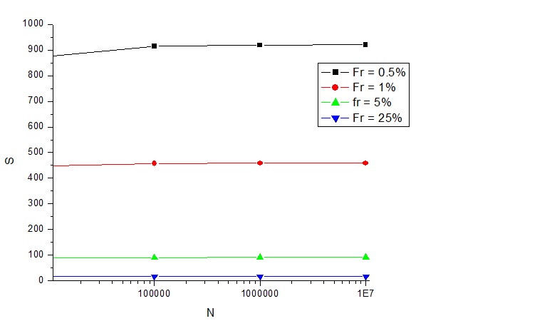
A very similar result can be obtained by plotting the above
hypergeometric distribution calculation for much larger populations of N:
Fig.1 above has been plotted for two rigging fractions 10% (with K
= 29) and 0.5% (with K = 534), as done by Prof.Atanu Biswas [1,3] – but
extrapolated to much higher values. The same tendency for 1 – P to saturate is
observed as in Van Dessel’s data [5] tabulated above. These kinds of results,
presumably, what Pof. Debasis Kundu is referring to as consequences of the
central limit theorem. The calculation can also be done for the case N =
1,800,000 and K = 1,000 and it gives P(X = 0) = 0.0066. This is a sampling
fraction (1/1,800 = 0.055%) very similar to what the Supreme Court finally
recommended, and smaller than what is obtained above (16,436/1,800,000 = 0.91%)
using Van Dessel’s online calculator [5].
Shetty [2] plots a similar saturation (Fig.2) in terms of the number
of samples required as the population size increases, assuming a hypergeometric
distribution.

The sampling fraction suggested by Prof.D.Kundu and the
Expert Committee does not agree with Unnikrishnan [8] or with Shetty [2]. The
critical point is this: should one treat each constituency separately as
done by Unnikrishnan and Shetty with only 3,134 EVMs or does one take the
whole lot (1,800,000 EVMs) in the entire country together? The results – in
terms of the sampling fraction – are very different: 16% as calculated by
Unnikrishnan [8,1] and <1 543="" a="" absolutely="" an="" any="" apparently="" argument="" as="" assumes="" being="" but="" central="" conceptual="" conclusive="" consequences.="" constituencies="" counter-intuitive="" course="" debasis="" difference:="" direction.="" do="" evm="" expert="" found="" has="" have="" i="" if="" in="" invokes="" is="" it="" just="" know.="" kundu="" leaning="" limit="" myself="" not="" o:p="" of="" one="" prof.="" randomly.="" rather="" real="" really="" s="" say="" saying="" selected="" tested="" that="" the="" theorem="" this="" to="" when="" world="" would="">
Since I could not figure it out I asked a statistician,
Prof.Chandan Mukherjee (Ambedkar University), and he pointed out that I was
implicitly assuming that all constituencies are identical. Not
only that they have the same number of EVMs (which is itself wrong, as
mentioned by Shetty [2]), but more importantly, that the level of rigging is
the same in each. Whereas it is more likely that only some constituencies
will be targeted, in which the results could go either way.
Prof.Mukherjee’s
argument would imply that the fraction recommended by Unnikrishnan [8] and by
Shetty [2] is right and each constituency must be considered separately.
That is, the number of EVMs currently mandated by the SC: 5 EVMs per
constituency is grossly inadequate.
In other words, the EC should follow Shetty’s
recommendations [2] rather than those of the Expert Committee.
(i)
The Hacking:
The statistical analysis simply decides how many EVMs should
be tested, assuming that we know how to detect a tampered EVM, no matter
what method was used to hack it. This may not always be the case.
However, the techniques used for hacking remain to be
discussed. Hari Prasad [9,10] claimed that several types of hacks are possible
and he wrote a paper along with his collaborators in 2010. Mainly, two methods
are used: a dishonest display is used to favour a particular candidate (by
changing the hardware of the EVM) or the vote is stolen by manipulating the
memory (by using a clip-on device to temporarily connect to the EVM). In the
former case, the hack is implemented by wirelessly communicating with the
pre-installed hardware inside the EVM, so it needs a small antenna, which,
Prasad claims can be hidden behind the circuit board of the EVM.
This specific claim is disputed by an engineer Dhiraj Sinha
[11] who argues that the smallest antenna that functions at GSM frequencies
(800/1800 MHz range) will be roughly 1x2x0.5 cm3in size, and it will
be even larger if lower frequencies are used (10X larger for 100 MHz) –
impossible to hide. Sinha also argues that it costs ‘millions of dollars’ to
design a chip and ‘hundreds of millions of dollars’ to actually implement it. Sinha’s
arguments are good – but not bullet-proof. After all, do the checkers open up
the EVM they are testing?
Amaldev [12] proposes a ‘sniffer’ hack which targets the 1.5
m long cable that connects the balloting unit (which the voter punches) to the
control unit (that actually records the vote). This hack involves replacing the
cable with another similar-looking cable and a small sniffer circuit. This hack
needs the help of EC officials at the booth, and it is possible to beat it by
inspecting the balloting unit to check if a sniffer circuit is attached to it.
Another vulnerability that has been pointed out [13] is that
the EVM chip is made by Renesas (Japan) and Microchip (USA): the one-time
programmable (OTP) microcontroller chip could be replaced abroad before being
shipped to India.
Prof.Poorvi Vora [14] has discussed some of the precautions
being taken by the EC:
a a) The EVM is a standalone unit, not connected to
the internet or to any network, which makes hacking difficult. But, as pointed
out, a sniffer circuit or an antenna could be used.
b b) Which EVM is allocated to which booth is done by
randomization. However, the randomization software and the seed used for
randomizing can be figured out by a hacker.
c c) EC uses cryptography to avoid attacks. But the
key used for encrypting can be figured out, or the data can be manipulated
before encryption.
d d) The EVMs are sealed before the candidate list is
decided, so a hacker will find it difficult to fix a specific button to favour
a given candidate – but there are ways to do this, it seems.
e e) A voter has about 6 seconds to view the VVPAT to
verify if the vote has been correctly registered. But, Prof.P.Vora points out,
the current protocol is that the vote gets registered anyway. The correct way
would have been to allow the voter to decide if the vote is correct, before it
is made final and recorded by the control unit.
In fact, former DGP Harekrishna Deka
noted that his vote was wrong [15] but did not make a complaint because he was
told that there was a fine and a 6 months jail sentence if he was proved wrong! EC has argued that this rule has been
introduced because a) otherwise they would be flooded with frivolous
complaints, and b) each such complaint would need 20 minutes to investigate,
which would hold up polling.
The fact that the chip is OTP is
an advantage, because once it is fused, according to an Expert Committee
Report: “it cannot be read, copied, altered or re-fed into the chip at all”.
Let’s give Prasad the last word on that:
“The point is, because of the masked code,
nobody can say with certainty that there cannot be built-in vulnerabilities in
the chip design,” said Prasad [9]. “Even if there is a vulnerability it will be
impossible for the Election Commission to detect. So, how do you rule out that
there cannot be another circuit designed within the chip?”
J.T. D’Souza adds:” Because the
OTP does not allow the code to be scrutinized, it is not possible to find out
if there was a Trojan or other vulnerability” [9]. There could be code embedded
within the EVM which only gets activated under specific circumstances (like one
specified candidate or party losing, or in response to a particular sequence/pattern of votes cast), that would not be detectable by normal
testing of the EVM.
Bottomline: India's EVMs are claimed to be foolproof. In principle, there is no such thing. In practice, the statistics being followed by EC at present - and even the 5 EVMs per constituency recommended by SC - seem to be inadequate. As far hacking methods go, there are many - and it would require extremely tight control by an independent, vigilant, open-minded and nimble body to prevent them all. Does the India's Election Commission really match these requirements?
2 2. K.Ashok Vardhan Shetty “Winning Voter
Confidence: Fixing India’s faulty VVPAT-based audit of EVMs“, The Hindu Centre
for Politics and Public Policy, Policy Watch Paper No.7, 2018
1 10.
Hari K.Prasad “Security analysis of India’s
Electronic Voting Machines” pdf document (29
th Apr.2010) at
http://IndiaEVM.org