Reactions to R0,
the SIR model and herd immunity
Nowadays, anybody with internet access who has read a couple
of papers fancies himself/herself to be an epidemiologist. As a physicist, by
training, I also want to jump in with my reactions to what little I have read,
to highlight the small fraction that (I think) I have understood.
Time Variations: exponential, logistic, SIR and SIRD
models:
In the initial phases the growth is exponential. In the
later phases, the growth slows down and can be fitted to the logistic curve, as
done by Rhett Allain [1,2], because there is only a finite population that the
virus can infect, while the exponential would keep going forever. Ranjan [2]
points out that the exponential curve predicts the initial build-up, but fails
to predict the eventual flattening out. The logistic curve:
I (t) = K/[ 1 + A exp(-rt)]
Where A = (K/I0) -1, reduces to the exponential
for small values of t:
I (t) = I0 exp(rt).
But the logistic curve, once fitted to the data, fails to
fit the initial time variation.
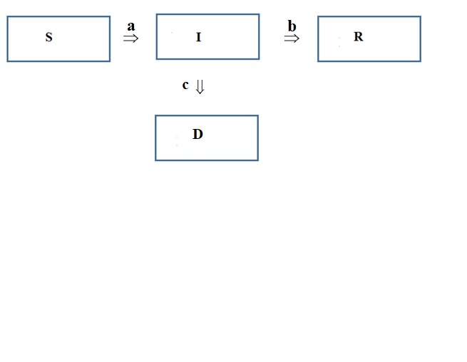
However, most epidemiologists follow the basic SIR model.
Proposed by Kermack & McKendrick [3], the model considers three categories
of people: those susceptible (S) to infection, those infected (I) and those who
have recovered (R). It is cast in terms of 3 coupled differential equations:
dS/dt = - a SI
dI/dt = aSI – b I
dR/dt = bI
where N is the population size, S is the number of
susceptible people, I is the number of infected people, R is the number of
recovered people, (such that N = S + I +R) , a is the infection rate (in units
of 1/day), b is the recovery rate (1/day) and c is the mortality rate (1/day). This
is expressed schematically in terms of transitions between compartments:

The basic SIR model was modified to take the probability of
death, after getting infected, into account, through the mortality rate c (1
/day), becoming the SIRD model by adding another differential equation and
adding one term to the dI/dt equation:
dS/dt = - a SI
dI/dt = aSI – (b +c)
I
dR/dt = bI
dD/dt = cI
such that N = S + I +R + D.
This is expressed in compartments as:
Basic Reproduction Number (BRN), R0:
But what of R0? According to Aronson et al [4],
the parameter R0 only characterizes the transmissibility, or the average
reproduction number, of the virus at the very beginning of the epidemic
in a homogeneous population (when there is zero immunity in the
population to the virus, so the whole population is susceptible).
The importance of R0 is that if it is less than
unity, the virus cannot spread (a physicist would call it ‘sub-critical’); but
if it is more than one, the virus multiples, exponentially (in
physicist-speak: avalanche
multiplication).
As the number of infected people changes, the
transmissibility decreases, and it is given by an effective reproduction rate Re.
This is related to R0 by the formula:
Re = R0 (1 – Pi),
where Pi
is the proportion of the population that is now immune to the virus – which
keeps increasing with time. But, to back up a bit, R0 is affected by
[3]:
(i)
The size of the population N, and the fraction
of the population that is susceptible at the beginning Ps(0) (Above Aronson said all are susceptible?)
(ii)
The infectiousness of the organism
(iii)
The recovery rate b (in the SIR model, recovery
includes death in addition to remission).
Both R0 and Re increases as N
increases, and as Ps(0) increases, and both decrease as the recovery rate b
increases. The effective reproduction rate Re is also affected by
the behavior of people e.g. physical distancing will decrease it.
According to Jones [5] and Delamater et al [6], it must be
emphasized that R0, the basic reproduction number (BRN), is dimensionless; it is often misleadingly characterized as a ‘rate’, which could only happen if it had
units of (time)-1:
R0 = tcavd
Where d is the duration of infectiousness (in days), cav
is the average rate of contact between susceptible and infected people (number/day)
and t is the transmissibility
of the infection, or the probability that the contact will result in infection.
Jones [5] also differentiates between R0 and Ri.
The first generation of an epidemic is all the secondary infections that result
from infectious contact with the index case, or generation zero. Ri
refers to the BRN of the ith generation, and R0 refers to
the number of infections generated by the index case (Gen zero). This is similar to the parameter Re mentioned
above [4]. The time between generations is called the serial interval, or the
average time between successive infections (1/b), or the number of infectious
days [7]. The problem with accurately estimating R0 is that,
initially, numbers are small and subject to statistical fluctuations. The
estimation of R0 is generally done by modeling and is tricky [5].
Similarly, Fernandez-Villaverde and Jones [8] express the
parameter R0 as a product of two variables in an intuitive way: it
is the product of the number of infectious days (1/b) and the number of (lengthy)
contacts per day (a) (or 1/a is the time between contacts):
R0 =
(1/b)(a).
Where a = tcav.
In the SIR model: R0 = a/b,
while in the SIRD
model: R0 = a/(b + c).
If there is no mortality, it reduces to the
SIR formula. The number of infectious days is characteristic of the virus, and
not controllable. But people can increase the time between contacts by social
distancing.
Ranjan [2] uses the formula:
R0 = (a/b) [1 – (I0/N)]
But initially I0 << N.
Similar to the above formula: Re = R0
(1 – Pi) is another formula (they are the same if we neglect the
recovered population) used by Caccavo in his SIRD model [9]:
Re = R0 (S/N)
Initially, S and N are almost the same, but as the number of
susceptible people decreases Re declines. The million dollar
question is: when does it hit one? That is the point in time at which the
number of infections peaks, and beyond that the epidemic dies out as Re
decreases further.
Herd Immunity:
The concept of herd immunity [4] was introduced in the
context of vaccination [10,11]. If a population is immunized above a threshold
H then the remainder of the population is given indirect protection, because
the infection/virus encounters too may immunized individuals and is unable to
propagate in the population. The herd immunity threshold is related to R0
by:
H = 1 – (1/R0)
For the case of covid-19, R0 is somewhere between
2.5 and 3.5, so the safe value of H is about 71% of the population, and about
29% of the population, though susceptible (never having been infected), will
remain protected from infection.
What is interesting is a different equation derived by
Bastin [11] and by Jones [5]. This relates R0 to the maximum
fraction xim of the population that ever gets infected, just before
the epidemic collapses to zero [11]:
R0 = - [ln(1 –xim)]/xim
Jones [5] expresses it equivalently in terms of the final susceptible fraction s¥:
ln (s¥)
= R0 (1 - s¥)
Bastin also gives an equation for the maximum value of
infected individuals, Imax:
Imax = N [1 – {{1 + ln(R0)}/R0}]
Bastin [11] even provides an I-S plot with an epidemic
trajectory:

The maximum number of infections occurs at the value of S =
b/a (or when Re = 1).
Compare this with the herd immunity threshold: H = 1 –
(b/a), and with the formula for the maximum number of s¥.
For simplicity, assume R0 = a/b = 3. The peak Imax
occurs when (S/N) = 1/3.
The herd immunity threshold is H = 2/3.
But what is the fraction s¥? it takes the value 0.06.
That is, the fraction of susceptible individuals is not 1/3 as expected from the herd
immunity formula but lower.
Here it is necessary to clarify: Bastin derives the formula
for xim in the context of a model that is different from the SIR
model mentioned above. Without going into details of his derivation, he introduces another
compartment called ‘exposed’, so it is now an SEIR model. A person who is
‘exposed’ has been exposed to the virus, but is not infectious yet. The SEIR
model takes into account the processes of births, deaths and vaccinations.
The question then really is: does herd immunity apply when
there is no vaccination? Can the infection itself be considered as equivalent
to vaccination, since the infected person is now immune to further infection
(never mind whether it was due to a live virus or an inactivated virus)?
The problem within the SIR model – which does not consider vaccination – is
that the infections continue beyond the herd immunity threshold, until s has
fallen to s¥
(see the Figure), at which point the number of infections drops to zero.
One might try to define the herd immunity threshold as the
point at which herd immunity just starts up, without really giving all of the
susceptible individuals immunity immediately - just an increasing level of immunity to more and more individuals as s approaches s¥. This is a consistent way of interpreting the
equations – but that is not what many prominent epidemiologists have claimed in
public. The advocates of herd immunity vocally state that all we have to do is
get 70% of the population infected, and the remaining 30% will be protected.
The advocates of this approach, initially in the U.K. and even today in Sweden
[4], argue that we need only isolate the elderly and the sick (with
co-morbidities), who have higher chances of dying than the young and healthy
majority (but see below!) According to Aronson et al
[4]:
“The problem with
leaving people to catch the infection spontaneously, leading to herd immunity,
would increase the death rate. For example, on 10 April, the number of
confirmed cases in Sweden was 9685 with 870 deaths (9.0%), compared with Norway
with 6219 confirmed cases and 108 deaths (1.7%) and Denmark with 5830 confirmed
cases and 237 deaths (4.4%).”
However, Aronson et al
[4] also argue:
“For example, if R0
= 2, immunization needs to be achieved in 50% of the population. However, if R0
= 5 the proportion rises steeply, to 80%. Beyond that the rise is less steep;
an increase in R0 to 10 (for measles) increases the need for
immunization to 90%.
When other children
become immune the infected child who encounters 10 children will not be able to
infect them all; the number infected will depend on Re. When
immunity is 90% or more the chances that the child will meet enough unimmunized
children to pass on the disease falls to near zero, and the population is
protected.” (emphasis added by me).
The point being made here is that the number to be infected
is higher: 94%, not 70% for R0 = 3. The lower and upper limits of R0
are also tabulated:
|
R0
|
(1/R0)
|
s¥
|
s¥ (from SIR program)
|
|
2.5
|
0.400
|
0.11
|
0.103
|
|
3
|
0.333
|
0.06
|
0.056
|
|
3.5
|
0.286
|
0.035
|
0.0306
|
|
5
|
0.200
|
0.007
|
0.00500
|
|
7
|
0.143
|
0.0008
|
0.00047
|
But look at the last 2 rows: for a high R0 of 5
only a very small fraction (0.7 %) is ‘protected’. And for even higher values,
that fraction becomes even smaller (0.05%).
So the question about the SIR vs the SEIR model
has real consequences.

The results of the SIR simulation (using Euler’s method
[11]) for R0 = 3 are similar to Bastin’s plot above. The arrow on
the S-axis indicates S¥
= 0.056. The arrow indicating the maximum has its position at S/N = 0.33 = 1/R0
as expected, and the value of the maximum is Imax = 3.07 x 10⁵,
close to the number expected (3.00 x 10⁵) from the equation for Imax
given above (by Bastin).
I just found an article by Prof. Gautam Menon [13] which
states that there are ‘sound methodological reasons’ to prefer the SEIR model
to the SIR model. Among others, the covid-19 has asymptomatic patients (the ‘E’
in SEIR) which SIR does not capture. More importantly, Menon states that the
SIR model: “predicts the numbers of
people with COVID-19 in India will decline immediately after a lockdown is
imposed. In contrast, an SEIR model would have predicted that the case load
would continue to increase before beginning to drop”.
There is plenty of criticism of the compartment models. For
example, Delamater et al [6] points out that R0 will fluctuate if
human-human or human-vector interactions vary with time and space. These
compartment models need to be modified to take into account the fact that
populations may be homogeneous or heterogeneous (e.g. different social classes
or age groups), that interactions are dynamic – either deterministic or
stochastic (with various possible distribution functions) – and pathogen
pathways may be complex involving intermediate hosts. In other words, some of
the basic simplifying assumptions made in early models have had to be modified
to take complex realities into account. Prof.Menon raises these concerns as
well [13].
Similar criticisms have been leveled by Huppert and Katriel
[14]:
a) the assumption of
“well-mixed populations” disregards the facts of geographical and social
proximity in enabling or preventing contacts
b) individuals are
different, some are more prone to infection, others may be more effective in
spreading infection (super-spreaders).
c) the duration of infection is assumed to be exponentially
distributed, but an individual need not become infectious immediately after
contracting an infection, and recovery from infection may depend upon how much
time has passed since getting infected.
d) populations are assumed to be large, so they can be treated
deterministically by differential equations; while small populations (a village
or a school) may be dominated by stochastic effects.
Menon [13] points out that there are other approaches than
the compartment model: a) an agent-based model b) Monte Carlo models c) purely
statistical or machine learning models d) network models.
Interestingly, Roda
et al [16] claim to have fitted the post-lockdown data in Wuhan to both SIR and
SEIR models, and say that the former is preferable, because the latter has too
many parameters that need to be estimated, and so the simpler SIR model is
better.
Regalado
[17] says that for an R0 of 3, 66% of the population has to be
immune before the effect (of herd immunity) ‘kicks in’, according to ‘the
simplest model’. Regalado is being careful, because herd immunity, even at 66%,
is not a free pass…
As a parting shot, note the following paragraph in a UK
newspaper [18]:
“About
60 per cent is the sort of figure you need to get herd immunity.” The
coronavirus won’t stop at 60 per cent, though, according to the British
scientists. Models promoted by Dr. Vallance and Britain’s chief medical
adviser, Chris Whitty, indicate that 80 per cent will ultimately become
infected. The trick is to limit that 80 per cent to those who can be safely
immunized, since infection for the others could mean death.
This is not the dominant narrative: see the characterization by Aronson et al above. Are epidemiologists just dumbing down the narrative for a public that they believe is incapable of understanding the details? But Chris Whitty did explain the details...
To
sum up: getting to 80% is harder than getting to 60%, since there are more
deaths along the way. The idea of herd immunity is not as attractive as it
seems to be at first sight.
References:
1.
Rhett Allain Wired 24th March
2020 https://www.wired.com/story/the-promising-math-behind-flattening-the-curve/
2.
Rajesh Ranjan,”Predictions for covid-19 outbreak
in India using epidemiological models,” 3rd April 2020 preprint: https://www.researchgate.net/publication/340314461
3.
W.O.Kermack and A.G.McKendrick Proc.Roy.Soc.
(Lond) A115 (1927) 700
4. J.K.Aronson
et al “’When will it be over?’: An introduction to viral reproduction
numbers, R0 and Re” www.cebm.net/oxford-covid-19/
5.
J.H.Jones “Notes
on R0” 1st
May 2007
https://web.stanford.edu/~jhj1/teachingdocs/Jones-on-R0.pdf
6.
P.L.Delamater et al, “Complexity of the Basic
Reproduction Number, R0” Emerging Infectious Diseases 15 (2019)
1 www.cdc.gov/eid
7.
Max Fisher, “R0, the messy metric,” https://www.nytimes.com/2020/04/23/world/europe/coronavirus-R0-explainer.html
8.
J.Fernandez-Villaverde and C.L.Jones, “
Estimating and simulating a SIRD model of Covid-19 for many countries, states
and cities,” 28th April 2020 Ver 0.6
9.
D.Caccavo, “Chinese and Italian outbreaks can be
correctly described by a modified SIRD model,”
17th Apr.2020 medRxiv preprint doi: https://doi.org/10.1101/2020.03.19.20039388
10.
P.E.M.Fine, “Herd immunity: history, theory,
practice”, Epidemiologic Rev. 15 (1993) 265
11.
G.Bastin, “Lectures on mathematical modeling of
biological systems,” 22nd Aug.2018 (GBIO 2060)
12.
Peter Adams,” Theory and Practice in
Science” https://people.smp.uq.edu.au/PeterAdams/SCIE1000/scie1000_notes_part2.pdf
13.
Gautam I.Menon https://science.thewire.in/the-sciences/covid-19-pandemic-infectious-disease-transmission-sir-seir-icmr-indiasim-agent-based-modelling/
14.
A.Huppert and G.Katriel,”Mathematical modeling
and prediction in infectious disease
epidemiology, “ Clinical Microbiology and Infection (Nov.2013) DOI:
10.1111/1469-0691.12308
15.
Gautam I.Menon https://science.thewire.in/the-sciences/coronavirus-pandemic-infectious-disease-transmission-modelling-kermack-mckendrick-theory-seir-model/
16.
W.C.Roda
et al, “Why is it difficult to accurately predict the covid-19 epidemic?”
Infectious Diseases Modeling 5 (2010) 271
17.
A.Regalado, “What is herd immunity and can it
stop the coronavirus?” 17th Mar 2020 https://www.technologyreview.com/2020/03/17/905244/what-is-herd-immunity-and-can-it-stop-the-coronavirus/
18.
Lawrence Solomon 16th March 2020,
“Britain’s approach to coronavirus: will herd immunity work?” https://www.theglobeandmail.com/opinion/article-britains-novel-approach-to-coronavirus-will-herd-immunity-work/
No comments:
Post a Comment