SIRD Simulations

SIRD simulations

Fig.1: Flattening the curve [1]

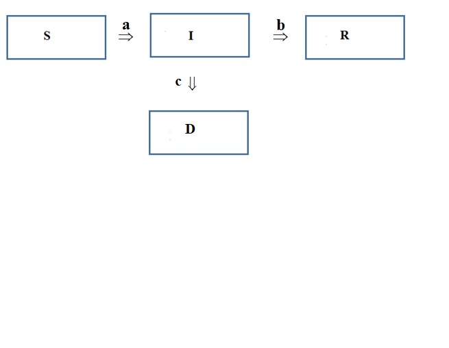
Carrying on from the last blog post, this post is about SIRD simulations. First, one attempts to do what has already been done before. Second, examine the parameters used by different authors. Finally, do some simulations, to look at the ‘D’ compartment: what values of mortality do SIRD models predict?

Fig.2: replicating Kumar [1]

Table: for N = 1x10⁶

R0	Infected proportion (Kumar et al)	Imax	Tmax (days)
1.862	0.129	135,000	39
1.455	0.055	57,300	65
1.258	0.023	23,200	101
1.2	0.015	15,000	124

Menon et al [2] have a similar plot, showing the effect of a lockdown, but there is much less change in the percentage of infected cases even after a 5-7 month lockdown than that shown by Kumar et al [1]:

Fig.3: from Menon et al [2]

However, the question of comparison arises again. The results of his SIR model are:

Fig.4: SIR simulation by Menon [2]

Numerically, Menon states that the maximum number infected is about 430 at about 4.77 days, and that only about 14 individuals out of a total of N = 1000 were uninfected at the end of 14 days. The parameters used were a = 2.18, b = 0.5 with only one infected individual at the start i.e. I(0) = 1 and S(0) = 999.

The results I get are a bit problematic because Euler’s method assumes differentiability and that’s a problem with such a small number of individuals. The closest I got to Menon’s results (by tweaking the interval) was I_max = 420 infected at 5.5 days and the uninfected number of individuals was about 10. Not very satisfactory. Note: Menon mentions using difference equations.

The general shape of the curves were similar (a small consolation):

Fig.5: replicating Menon’s SIR simulation [2]

Apart from these results from the SIR model, what is of more interest is the SIRD model [3]. Adams considers the 1918 flu, and assumes N = 1x10⁶, a = 1.9 per week, b = 1.4 per week and c = 0.065 per week. The epidemic he plots over a period of 45 weeks.

The results obtained by me are within 2% of those of Adams:

	Adams	Mine
No. of deaths	19,200	18,755
Imax	29,800	29,152
Rmax	435,000	403,970
Tmax (weeks)	27.6	27.6

The shape of the plots is very close as you would expect from the table, so I have not used Adam’s plots. First the I-D plot vs time (in weeks):

Fig.6: from Adams [3]

And the S-R plot (with time in weeks):

Fig7: from Adams [3]

The question is what values of a, b & c should be used? First look at the table below:

	a (d-1)	b (d-1)	c (d-1)	R0
Adams (SIRD)	0.271	0.20	0.0093	1.295
Anastassopoulou (SIRD)	0.191 0.319	0.064 (~1/15) 0.16	0.01 0.0005	2.581 2
Caccavo (modified SIRD)	0.553 0.256	0.076 0.017	0.009 0.024	6.505
Ferguson (agent-based & SEIR)	-	-	-	2, 2.2, 2.4, 2.6
Karin (SEIR)	0.95; 0.5 & 0.7	0.25; 0.163	-	3.8; 2.0;  2.8
Van Wees (SEIR)	1.75	0.5		3.5
Walker (SEIR)	0.478 (1/(2.09)) ??	0.2 (1/5)	0.0476 (1/21)	3.0
Volz (SEIR)		(1/6.5)		2.9
Bertozzi (SIR)	0.26 – 0.41	0.10, 0.12	-	2.1-4.6
Guttal (10 comp. model)	0.42	0.1428	0.0136	~2.7 1.8 with social distancing
Lin (SEIR + 2c)	0.5944	0.2	-	2.8
Alvarez (SIR)	0.2	0.0555 (1/18)		3.6
Chinazzi	(1/6 – 1/11)			2.57
Li	1/7.5			2.2

Many of these are SIR models, or SEIR, or agent-based. In some cases, more than one set of values has been given. Note that the values given by Adams are for the 1918 flu, whereas all the rest are for covid-19.

The recovery period has been taken by most as the mean incubation of 5.2 days, but the value of b has been calculated in many cases by assuming a total hospitalization period of about 12.4 days. The reason for this difference is that the incubation period is to be used in the SEIR models for the E Þ I, transition, while in the SIR or SIRD model, the S Þ I transition should take the average hospitalization period into account. Thus, the value of b should be ~ 0.08. This point is also made by Atkeson [14], except that he uses the value of 18 days instead of 12.4 days (citing a paper from China, by Wang [15]).

Note, however, Lin et al [16] have used b = 0.2, citing another paper by Nishiura [17] that states that the serial interval is 5 days (i.e. the time between generations). Chinazzi [18] quotes a range of 6-11 days for the generation time, and a R₀ of 2.57, corresponding to a doubling time T_d of 4.2 days. 

Whereas, Li [19] estimated 7.5 days for the serial interval, with R₀ = 2.2 and a mean incubation period of 5.2 days.

The value of ‘a’ should be in the range 0.2-0.55. Alvarez [20] uses a value of a = 0.2.

According to Du et al [20], the value of R₀ is estimated for an epidemic in its initial stages from its growth rate r, the mean generation time m and the standard deviation s of its generation time, assuming normally distributed generation times:

R₀ = exp(mr – {s²r²/2})

Caccavo [5] has quoted two sets of values, the first set for China, and the second for Italy. However, he introduces a modification that the parameter c is time-dependent, decreasing exponentially with a time constant of t_c  = 21.6 days:

c = c₀ exp(-t/t_c)

Actually, to fit the Chinese data he also added similar time constants for the parameters a and b. He claims that his plots fit the data correctly, and he gets the number of deaths in Italy right.

Amidst all this uncertainty, Park et al [22] attempted to reconcile differing estimates of the basic reproductive number R₀ by using a ‘multi-level Bayesian framework’. They argue that R₀ depends on 3 parameters: the exponential growth rate r (in the initial phases), the mean generation interval G_m and the dispersion k in the generation interval. After their statistical analysis of six independent studies, they concluded with a median value for the basic reproductive number of R₀ = 2.9, with a range of 2.1 to 4.5 with 95% confidence.

However, when all is said and done, Biswas [23] argues that we should ‘keep it retrospective’. He accepts that policy-makers need guidance based on evidence, but is skeptical about the possibility of prediction, considering the varying models and the uncertainties in parameters. This view is shared by Adam [24]: “much information about how SARS-COV-2 spreads is still unknown and must be estimated or assumed and that limits the precision of forecasts.” Adam quotes a paper by the group of John Edmunds [25] that assessed the performance of models in a 2014-15 Ebola outbreak in Sierra Leone, and found that it was possible to reliably predict the course of the epidemic up to 2 weeks, but no more than that. In addition, the difficulty of determining the value of R₀ has to do with the fact that many of the early values are small numbers (to determine the growth rate r) and are thus subject to statistical fluctuations. These can be tamed to some extent by using moving averages over many days, but it is more of a problem for deaths than for infected cases [26], since the numbers are smaller.

What of the mortality rate c? It may be as low as 0.0005, or as high as 0.05, but a mean value of 0.01 may be taken. With all this uncertainty, this range of parameters seems par for the course. Mortality estimates for covid-19 have varied between 0.6% and 1.4% of those who get infected [27]. Maybe one can get some number within this range by plugging in values of a, b and c in the SIRD model.

Let us first fix b as 1/7.5 = 0.133 based on the generation time given by Li [19]. Chinazzi [18] quotes a range of 6-11 days. Anastassopoulou et al [4] give two values, but one value is b = 0.16. Let us use the two values of c given by [4] 0.01 and 0.0005. The value of a can be taken as a variable corresponding to the range of R₀ of 2.0 to 3.5 which covers most of the values in the above table.

First, assume b = 0.064 and c = 0.0005 (all for N = 1x10⁶):

R0	S¥	R¥	D¥	Imax
2	199,552	794,252	6,205	155,714
2.5	103,320	889,836	6,952	238,070
3	55,563	937,125	7,321	307,460
3.5	30,558	961,935	7,515	366,393
5	5,259	987,039	7,711	490,750
10	8	992,249	7,752	677,644

Next, assume b = 0.064 and c = 0.0025:

R0	S¥	R¥	D¥	Imax
2	199,438	770,475	30,097	155,839
2.5	103,090	863,200	33,710	237,990
3	55,438	909,061	35,510	307,469
3.5	30,449	933,110	36,449	365,312
5	5,207	957,404	37,398	494,829
10	7	962,408	37,594	704,384

And then, assume b = 0.064 and c = 0.01:

R0	S¥	R¥	D¥	Imax
2	199,009	692,758	108,243	155,921
2.5	102,600	776,138	121,271	238,553
3	54,969	817,331	127,708	308,742
3.5	30,041	838,890	131,077	367,844
5	5,013	860,537	134,459	496,402
10	5	864,868	135,135	677,479

A look at the above tables shows that c does not affect S_¥ or I_max much, but the effect is stronger on R_¥ and greatest on D_¥. Increasing R₀ decreases S_¥ and increases R_¥ as expected, while also increasing D_¥ and increasing I_max.

A further examination of at the above tables would suggest that, as R₀ increases (beyond 3.5), R_¥ and D_¥ saturate. That is, beyond a point, increasing transmissibility does not result in increasing fatalities. However, I_max continues to increase, but does not show consistent variation.

The standard plot of S, I and R vs time (in days) is:

Fig.8:

While the plot that shows the dead (a smaller number) along with those infected is:

Fig.9:

First, assume b = 0.133 and c = 0.0005 (all for N = 1x10⁶):

R0	S¥	R¥	D¥	Imax
2	195,547	801,449	3,013	158,112
2.5	98,633	898,000	3,376	241,569
3	51,176	945,280	3,554	315,024
3.5	26,759	969,606	3,645	369,667
5	3,537	992,740	3,732	498,996
10	0	996,264	3,745	680.429

Next, assume b = 0.133 and c = 0.0025:

R0	S¥	R¥	D¥	Imax
2	195,430	789,735	14,845	158,350
2.5	98,497	884,880	16,633	241,201
3	51,046	931,455	17,508	313,489
3.5	26,647	955,404	17,959	375,871
5	3,490	978,134	18,386	510,052
10	0	981,560	18,450	710,875

And then, assume b = 0.133 and c = 0.01:

R0	S¥	R¥	D¥	Imax
2	194,986	748,728	56,295	158,071
2.5	97,987	838,944	63,078	241,818
3	50,558	883,056	66,395	316,274
3.5	26,227	905,686	68,097	376,332
5	3,313	926,997	69,699	481,408
10	0	930,079	69,930	619,992

The SIR model prediction is from Bastin [28]:

R₀ = - [ln(1-x)]/x

where x = 1 – (S_¥/N).

You would expect the SIRD model to deviate from the SIR model prediction and it does:

R0	X	1 – (S¥/N)	1 – (S¥/N)	1 – (S¥/N)	1 – (S¥/N)
2	0.800	0.800	0.804	0.800	0.805
2.5	0.890	0.897	0.901	0.8974	0.902
3	0.9403	0.9444	0.9488	0.9450	0.9494
3.5	0.9659	0.9694	0.9732	0.9700	0.9738
5	0.9930	0.9947	.9965	0.9950	0.9967
		b = 0.064	b = 0.133	b = 0.064	b = 0.133
		c = 0.0005		c  = 0.01

But the deviation is not all that great, except that it goes up as R₀ increases, and also as b and c increase, with the largest deviation being for the highest value of all three parameters.

The SIR formula for I_max is [28]:

I_max = N[ 1- {1+ ln(R₀)}/R₀]

For N = 1x10⁶:

R0	Imax
2	153,426
2.5	233,484
3	300,462
3.5	356,353
5	478,112
10	669,741

From R_¥ and D_¥ in the above tables we can estimate the percentage of deaths among those who were infected:

C	b = 0.064	b = 0.133
0.0005	0.78%	0.37%
0.0025	3.76%	1.84%
0.01	13.51%	6.99%

This percentage does not seem to depend much on the value of R₀ (in the range 2-5), but it clearly depends on the value of b and c.  The value of b = 0.064 predicts a high percentage, since recovery takes a long time, 15.6 days (i.e. it is less effective as a mechanism). The column with b = 0.133 looks somewhat better, but clearly a lot depends on the assumed value of the parameter c. If c is low, mortality is an ineffective mechanism. However, is a value of 0.0025 (corresponding to 400 days) reasonable? With this set of parameters, it is the only way to get about 1.8%. And the lower end value of 0.0005 (2,000 days) looks even more questionable.

However, let us do a reality check. The population of Italy is about 60.4 million. According to [29], the toll in Italy is 228,006 cases and 32,406 deaths on 23^rd May 2020. The paper of Anastassopoulou et al [4] considers two sets of parameters: (i) a = 0.191, b = 0.064 and c = 0.01, and (ii) a = 0.319, b = 0.16 and c = 0.0005. Case (i) corresponds to R₀ = 2.58, while case (ii) is for R₀ = 1.98. We prefer case (ii), since the recovery period of 6.25 days seems more reasonable than the recovery time of 15.6 days. Even for case (ii), the number of deaths (per million) is 2,500. Multiply by 60, and this gives 150,000 deaths – which is about 5X the actual value to date. Note, however, that Anastassopoulou et al [4] have fitted their data to Wuhan in China, not Italy.  

Anastassopoulou et al [4] also consider values of a, b and c taking into account the confidence intervals in their determination. According to them, a is estimated to a high level of accuracy (0.319 ±0.001 and 0.191 ±0.001) but they take a ±10% variation in the parameters b and c. This would be fine, except for the fact that the two sets of parameters (i) and (ii) differ to such a great extent. The authors explain that the second data set has been calculated assuming that the data from China underestimated the number of infected cases by 20X and the number of recovered cases by 40X, but was accurate in estimating the number of deaths.

Of course, there are problems with these arguments: assuming the same value of a, b and c throughout does not take into account the efforts of lockdown and social distancing. A more sophisticated analysis would be needed for that, with time-varying parameters, as was done by Caccavo [5]. Further, as pointed out earlier, this analysis disregards spatial inhomogeneity: North Italy was much more seriously affected than South Italy. It also does not take into account the higher mortality of old people and the age-structure of the population.  So it is possible that the second set of values chosen [4] is actually reasonable – if you also factor in time- and space-variations. However, models can get very complicated; INDSCI-SIM of Guttal et al [30] has a 9 compartment model, while Menon et al [2] have a 10-compartment model. And complicated models are ‘data-hungry’. Even with the internet, getting hold of all the data … easier said than done.

 Fig.10: from Menon [2]

Worryingly, Menon et al [2] have a plot showing that 10% of the population in India will be dead within a year – despite the lockdowns. This percentage is significantly larger than even the highest value in the table above (13.5%). They have a number of policy prescriptions for eradicating the virus (apart from a vaccine), but they do not discuss the effect of these prescriptions on mortality. And following the complexities of a 10-compartment model is beyond me…

However, bottom-line is that if one uses Caccavo’s parameters for Italy [5] one winds up with 3.2% of the population dead. While this is still high, it is a lot better than Menon’s value of 10%! However, Caccavo’s value of b (0.017; 58 days) [5] does not seem to be particularly reasonable. If one were to use b = 0.133, as discussed above, (while keeping a, c₀ and t_c the same, 0.256, 0.024 & 21.6 respectively) the fraction of people that drop dead, drops down to 0.17%! Which would be an outcome that would be significantly better.

However, as Biswas {23] says, better ‘keep it retrospective’, a view that would be endorsed by Adam [24] and Edmunds [25]: post-diction is easier than prediction.

References:

1  1.     Kaushalendra Kumar, Wahengbam Bigyananda Meitei and Abhishek Singh “Projecting the future trajectory of COVID-19 infections in India using the susceptible-infected-recovered (SIR) model” IIPS Analytical Series on Covid 19: Paper 7

2  2.      Ashish Menon, Nithin K Rajendran, Anish Chandrachud, Girish Setlur “Modelling and simulation of COVID-19 propagation in a large population with specific reference to India,” medRxiv preprint doi: https://doi.org/10.1101/2020.04.30.20086306; this version posted May 5, 2020

3  3.     Peter Adams,” Theory and Practice in Science”  https://people.smp.uq.edu.au/PeterAdams/SCIE1000/scie1000_notes_part2.pdf

4 4.   C.Anastassopoulou, L.Russo, A.Tsakris and C.Siettos 31^st March 2020 PlosOne  https://doi.org/10.1371/journal.pone.0230405

5 5.   D.Caccavo medRxiv 17Apr2020  https://doi.org/10.1101/2020.03.19.20039388

6 6.   N.M.Ferguson et al  Nature Vol 442|27 July 2006|doi:10.1038/nature04795

7 7.   O.Karin et al, “Adaptive cyclic exit strategies from lockdown to suppress

COVID-19 and allow economic activity,”medRxiv doi: https://doi.org/10.1101/2020.04.04.20053579

8 8.    J.-D.Van Wees et al, “Forecasting hospitalization and ICU rates of the COVID-19 outbreak: an efficient SEIR model,” Bull World Health Organ. E-pub: 30 March 2020. doi: http://dx.doi.org/10.2471/BLT.20.256743

9 9.   P.G.T.Walker et al, “Report 12: The Global Impact of COVID-19 and Strategies for Mitigation and Suppression  ,”26^th Mar.2020 DOI: https://doi.org/10.25561/77735

1 10.   E.Volz et al, “Report 5: Phylogenetic analysis of SARS-CoV-2  ,”  15^th Feb.2020  DOI: https://doi.org/10.25561/77169

1 11.   A.L.Bertozzi et al,  “The challenges of modeling and forecasting the spread of COVID-19,” arXiv 9Apr 2020 2004.04741v1

1 12.   V.Guttal et al  “INDSCI-SIM: a state-level epidemiological model for India,” 18^th Apr.2020

 113.   A.Biswas, “A prediction model for covid-19”, 17^th March 2020 https://www.thehindu.com/opinion/op-ed/a-prediction-model-for-covid-19/article31092695.ece

1  14.   A.Atkeson “What will be the economic impact of Covid-19 in the U.S.? Rough estimates  of disease scenarios,“NBER Working Paper 26867 March 2020    

1  15.   H.Wang et al, “Phase-adjusted estimation of number of coronavirus disease 2019 cases in Wuhan, China,”  Cell Discovery 6 (2020) 10;  https://doi.org/10.1038/s41421-020-0148-0

1  16.   Q.Lin et al , “ A conceptual model for the outbreak of coronavirus disease (Covid-19) in Wuhan, China, with individual reaction and governmental action”, Int.J.Inf.Dis. 93 (2020) 211

1  17.   H.Nishiura et al, “Serial interval of novel coronavirus (covid-19) infections,” Int.J.Inf.Dis. 93 (2020) 284

    18.   M.Chinazzi et al, “The effect of travel restrictions on the spraed of the 2019 novel coronoavirus (COVID-19) outbreak,” Science 368 (2020) 394 24^th Apr.2020

1  19.   Q.Li et al, “Early transmission dynamics in Wuham China, of novel corononavirus-infected pneumonia,” New England J.Med. 382 (2020) 26^th Mar 2020 1199 DOI: 10.1056/NEJMoa2001316

2  20.   F.E.Alvarez, “A simple planning problem for covid-19 lockdown,” NBER Working Paper 26981 April 2020

2  21.   Z.Du et al ,” The serial interval of covid-19 from publicly confirmed cases,” medRxiv 20^th Mar 2020 https://doi.org/10.1101/2020.02.19.20025452

2  22.   S.W.Park et al ,”Reconciling early outbreak estimates of basic reproductive number and its uncertainty,” medRxiv 28^th Feb.2020 doi: https://doi.org/10.1101/2020.01.30.20019877

2  23.   A.Biswas, “Keep it retrospective,” Hindu, 21^st May 2020.

2  24.   D.Adam, ”Modelling the pandemic,”  Nature 580 (16^th April 2020) 316

2  25.   S.Funk et al ,” Assessing the performance of real-time epidemic forecasts,” PLOS Computational  Biol. https://doi.org/10.1371/journal.pcbi.1006785

2  26.   S.Ramesh & M.Basu, https://theprint.in/science/r0-data-shows-indias-coronavirus-infection-rate-has-slowed-gives-lockdown-a-thumbs-up/399734/

    27.   Prof.Devi Sridhar https://www.theguardian.com/commentisfree/2020/apr/08/how-will-the-coronavirus-crisis-end-lockdown-pandemic

2  28.   S.Bastin, “Lectures on mathematical modelling of biological systems,” 22^nd Aug.2018, GBIO 2060

https://perso.uclouvain.be/georges.bastin/lectures-bio.pd

2 29.   https://www.worldometers.info/coronavirus/country/italy/

3 30.   V.Guttal et al a) medRxiv 1^st May 2020 doi: https://doi.org/10.1101/2020.04.26.20080648

and b) INDSCI-SIM: a State-level epidemiological model for India 18^th April 2020 www.indscicov.in

Reactions to R0, the SIR model and herd immunity

Reactions to R₀, the SIR model and herd immunity

Nowadays, anybody with internet access who has read a couple of papers fancies himself/herself to be an epidemiologist. As a physicist, by training, I also want to jump in with my reactions to what little I have read, to highlight the small fraction that (I think) I have understood.

Time Variations: exponential, logistic, SIR and SIRD models:

In the initial phases the growth is exponential. In the later phases, the growth slows down and can be fitted to the logistic curve, as done by Rhett Allain [1,2], because there is only a finite population that the virus can infect, while the exponential would keep going forever. Ranjan [2] points out that the exponential curve predicts the initial build-up, but fails to predict the eventual flattening out. The logistic curve:

I (t) = K/[ 1 + A exp(-rt)]

Where A = (K/I₀) -1, reduces to the exponential for small values of t: 

I (t) = I₀ exp(rt).

But the logistic curve, once fitted to the data, fails to fit the initial time variation.

However, most epidemiologists follow the basic SIR model. Proposed by Kermack & McKendrick [3], the model considers three categories of people: those susceptible (S) to infection, those infected (I) and those who have recovered (R). It is cast in terms of 3 coupled differential equations:

dS/dt = - a SI

dI/dt = aSI – b I

dR/dt = bI

where N is the population size, S is the number of susceptible people, I is the number of infected people, R is the number of recovered people, (such that N = S + I +R) , a is the infection rate (in units of 1/day), b is the recovery rate (1/day) and c is the mortality rate (1/day). This is expressed schematically in terms of transitions between compartments:

The basic SIR model was modified to take the probability of death, after getting infected, into account, through the mortality rate c (1 /day), becoming the SIRD model by adding another differential equation and adding one term to the dI/dt equation:

   dS/dt = - a SI

dI/dt = aSI – (b +c)  I

dR/dt = bI

dD/dt = cI

such that N = S + I +R + D.

This is expressed in compartments as:

Basic Reproduction Number (BRN), R₀:

But what of R₀? According to Aronson et al [4], the parameter R₀ only characterizes the transmissibility, or the average reproduction number, of the virus at the very beginning of the epidemic in a homogeneous population (when there is zero immunity in the population to the virus, so the whole population is susceptible).

The importance of R₀ is that if it is less than unity, the virus cannot spread (a physicist would call it ‘sub-critical’); but if it is more than one, the virus multiples, exponentially (in physicist-speak:  avalanche multiplication).

As the number of infected people changes, the transmissibility decreases, and it is given by an effective reproduction rate R_e. This is related to R₀ by the formula:

R_e = R₀ (1 – P_i), 

where P_i is the proportion of the population that is now immune to the virus – which keeps increasing with time. But, to back up a bit, R₀ is affected by [3]:

(i)                  The size of the population N, and the fraction of the population that is susceptible at the beginning P_s(0) (Above Aronson said all are susceptible?)

(ii)                The infectiousness of the organism

(iii)               The recovery rate b (in the SIR model, recovery includes death in addition to remission).

Both R₀ and R_e increases as N increases, and as P_s(0) increases, and  both decrease as the recovery rate b increases. The effective reproduction rate R_e is also affected by the behavior of people e.g. physical distancing will decrease it.

According to Jones [5] and Delamater et al [6], it must be emphasized that R₀, the basic reproduction number (BRN), is dimensionless; it is often misleadingly characterized as a ‘rate’, which could only happen if it had units of (time)^-1:

R₀ = tc_avd

Where d is the duration of infectiousness (in days), c_av is the average rate of contact between susceptible and infected people (number/day) and t is the transmissibility of the infection, or the probability that the contact will result in infection.

Jones [5] also differentiates between R₀ and R_i. The first generation of an epidemic is all the secondary infections that result from infectious contact with the index case, or generation zero. R_i refers to the BRN of the i^th generation, and R₀ refers to the number of infections generated by the index case (Gen zero).  This is similar to the parameter R_e mentioned above [4]. The time between generations is called the serial interval, or the average time between successive infections (1/b), or the number of infectious days [7]. The problem with accurately estimating R₀ is that, initially, numbers are small and subject to statistical fluctuations. The estimation of R₀ is generally done by modeling and is tricky [5].

Similarly, Fernandez-Villaverde and Jones [8] express the parameter R₀ as a product of two variables in an intuitive way: it is the product of the number of infectious days (1/b) and the number of (lengthy) contacts per day (a) (or 1/a is the time between contacts):

 R₀ = (1/b)(a).

Where a = tc_av.

In the SIR model: R₀ = a/b, 

while in the SIRD model: R₀ = a/(b + c). 

If there is no mortality, it reduces to the SIR formula. The number of infectious days is characteristic of the virus, and not controllable. But people can increase the time between contacts by social distancing.

Ranjan [2] uses the formula:

R₀ = (a/b) [1 – (I₀/N)]

But initially I₀ << N.

Similar to the above formula: R_e = R₀ (1 – P_i) is another formula (they are the same if we neglect the recovered population) used by Caccavo in his SIRD model [9]:

R_e = R₀ (S/N)

Initially, S and N are almost the same, but as the number of susceptible people decreases R_e declines. The million dollar question is: when does it hit one? That is the point in time at which the number of infections peaks, and beyond that the epidemic dies out as R_e decreases further.

Herd Immunity:

The concept of herd immunity [4] was introduced in the context of vaccination [10,11]. If a population is immunized above a threshold H then the remainder of the population is given indirect protection, because the infection/virus encounters too may immunized individuals and is unable to propagate in the population. The herd immunity threshold is related to R₀ by:

H = 1 – (1/R₀)

For the case of covid-19, R₀ is somewhere between 2.5 and 3.5, so the safe value of H is about 71% of the population, and about 29% of the population, though susceptible (never having been infected), will remain protected from infection.

What is interesting is a different equation derived by Bastin [11] and by Jones [5]. This relates R₀ to the maximum fraction x_im of the population that ever gets infected, just before the epidemic collapses to zero [11]:

R₀ = - [ln(1 –x_im)]/x_im

Jones [5] expresses it equivalently in terms of the final susceptible fraction s_¥:

ln (s_¥) = R₀ (1 - s_¥)

Bastin also gives an equation for the maximum value of infected individuals, I_max:

I_max = N [1 – {{1 + ln(R₀)}/R₀}]

Bastin [11] even provides an I-S plot with an epidemic trajectory:

The maximum number of infections occurs at the value of S = b/a (or when R_e = 1).

Compare this with the herd immunity threshold: H = 1 – (b/a), and with the formula for the maximum number of s_¥.

For simplicity, assume R₀ = a/b = 3. The peak I_max occurs when (S/N) = 1/3.

The herd immunity threshold is H = 2/3.

But what is the fraction s_¥? it takes the value 0.06. That is, the fraction of susceptible individuals is not 1/3 as expected from the herd immunity formula but lower.

Here it is necessary to clarify: Bastin derives the formula for x_im in the context of a model that is different from the SIR model mentioned above. Without going into details of his derivation, he introduces another compartment called ‘exposed’, so it is now an SEIR model. A person who is ‘exposed’ has been exposed to the virus, but is not infectious yet. The SEIR model takes into account the processes of births, deaths and vaccinations.

The question then really is: does herd immunity apply when there is no vaccination? Can the infection itself be considered as equivalent to vaccination, since the infected person is now immune to further infection (never mind whether it was due to a live virus or an inactivated virus)?

The problem within the SIR model – which does not consider vaccination – is that the infections continue beyond the herd immunity threshold, until s has fallen to s_¥ (see the Figure), at which point the number of infections drops to zero.

One might try to define the herd immunity threshold as the point at which herd immunity just starts up, without really giving all of the susceptible individuals immunity immediately - just an increasing level of immunity to more and more individuals as s approaches s_¥.  This is a consistent way of interpreting the equations – but that is not what many prominent epidemiologists have claimed in public. The advocates of herd immunity vocally state that all we have to do is get 70% of the population infected, and the remaining 30% will be protected. The advocates of this approach, initially in the U.K. and even today in Sweden [4], argue that we need only isolate the elderly and the sick (with co-morbidities), who have higher chances of dying than the young and healthy majority (but see below!) According to Aronson et al [4]:

“The problem with leaving people to catch the infection spontaneously, leading to herd immunity, would increase the death rate. For example, on 10 April, the number of confirmed cases in Sweden was 9685 with 870 deaths (9.0%), compared with Norway with 6219 confirmed cases and 108 deaths (1.7%) and Denmark with 5830 confirmed cases and 237 deaths (4.4%).”

However, Aronson et al [4] also argue:

“For example, if R₀ = 2, immunization needs to be achieved in 50% of the population. However, if R₀ = 5 the proportion rises steeply, to 80%. Beyond that the rise is less steep; an increase in R₀ to 10 (for measles) increases the need for immunization to 90%.

When other children become immune the infected child who encounters 10 children will not be able to infect them all; the number infected will depend on R_e. When immunity is 90% or more the chances that the child will meet enough unimmunized children to pass on the disease falls to near zero, and the population is protected.” (emphasis added by me).

The point being made here is that the number to be infected is higher: 94%, not 70% for R₀ = 3. The lower and upper limits of R₀ are also tabulated:

R0	(1/R0)	s¥	s¥ (from SIR program)
2.5	0.400	0.11	0.103
3	0.333	0.06	0.056
3.5	0.286	0.035	0.0306
5	0.200	0.007	0.00500
7	0.143	0.0008	0.00047

But look at the last 2 rows: for a high R₀ of 5 only a very small fraction (0.7 %) is ‘protected’. And for even higher values, that fraction becomes even smaller (0.05%).

So the question about the SIR vs the SEIR model has real consequences.

The results of the SIR simulation (using Euler’s method [11]) for R₀ = 3 are similar to Bastin’s plot above. The arrow on the S-axis indicates S_¥ = 0.056. The arrow indicating the maximum has its position at S/N = 0.33 = 1/R₀ as expected, and the value of the maximum is I_max = 3.07 x 10⁵, close to the number expected (3.00 x 10⁵) from the equation for I_max given above (by Bastin).

I just found an article by Prof. Gautam Menon [13] which states that there are ‘sound methodological reasons’ to prefer the SEIR model to the SIR model. Among others, the covid-19 has asymptomatic patients (the ‘E’ in SEIR) which SIR does not capture. More importantly, Menon states that the SIR model: “predicts the numbers of people with COVID-19 in India will decline immediately after a lockdown is imposed. In contrast, an SEIR model would have predicted that the case load would continue to increase before beginning to drop”.

There is plenty of criticism of the compartment models. For example, Delamater et al [6] points out that R₀ will fluctuate if human-human or human-vector interactions vary with time and space. These compartment models need to be modified to take into account the fact that populations may be homogeneous or heterogeneous (e.g. different social classes or age groups), that interactions are dynamic – either deterministic or stochastic (with various possible distribution functions) – and pathogen pathways may be complex involving intermediate hosts. In other words, some of the basic simplifying assumptions made in early models have had to be modified to take complex realities into account. Prof.Menon raises these concerns as well [13].

Similar criticisms have been leveled by Huppert and Katriel [14]:

a)  the assumption of “well-mixed populations” disregards the facts of geographical and social proximity in enabling or preventing contacts

b)  individuals are different, some are more prone to infection, others may be more effective in spreading infection (super-spreaders).

c) the duration of infection is assumed to be exponentially distributed, but an individual need not become infectious immediately after contracting an infection, and recovery from infection may depend upon how much time has passed since getting infected.

d) populations are assumed to be  large, so they can be treated deterministically by differential equations; while small populations (a village or a school) may be dominated by stochastic effects.

Menon [13] points out that there are other approaches than the compartment model: a) an agent-based model b) Monte Carlo models c) purely statistical or machine learning models d) network models. 

Interestingly, Roda et al [16] claim to have fitted the post-lockdown data in Wuhan to both SIR and SEIR models, and say that the former is preferable, because the latter has too many parameters that need to be estimated, and so the simpler SIR model is better.

Regalado [17] says that for an R₀ of 3, 66% of the population has to be immune before the effect (of herd immunity) ‘kicks in’, according to ‘the simplest model’. Regalado is being careful, because herd immunity, even at 66%, is not a free pass…

As a parting shot, note the following paragraph in a UK newspaper [18]:

“About 60 per cent is the sort of figure you need to get herd immunity.” The coronavirus won’t stop at 60 per cent, though, according to the British scientists. Models promoted by Dr. Vallance and Britain’s chief medical adviser, Chris Whitty, indicate that 80 per cent will ultimately become infected. The trick is to limit that 80 per cent to those who can be safely immunized, since infection for the others could mean death.

This is not the dominant narrative: see the characterization by Aronson et al above. Are epidemiologists just dumbing down the narrative for a public that they believe is incapable of understanding the details? But Chris Whitty did explain the details... 

To sum up: getting to 80% is harder than getting to 60%, since there are more deaths along the way. The idea of herd immunity is not as attractive as it seems to be at first sight.

References:

1.       Rhett Allain Wired 24^th March 2020 https://www.wired.com/story/the-promising-math-behind-flattening-the-curve/

2.       Rajesh Ranjan,”Predictions for covid-19 outbreak in India using epidemiological models,” 3^rd April 2020     preprint: https://www.researchgate.net/publication/340314461

3.       W.O.Kermack and A.G.McKendrick Proc.Roy.Soc. (Lond) A115 (1927) 700

4.       J.K.Aronson et al “’When will it be over?’: An introduction to viral reproduction

numbers, R₀ and R_e” www.cebm.net/oxford-covid-19/

5.       J.H.Jones “Notes  on R₀”  1^st May 2007

https://web.stanford.edu/~jhj1/teachingdocs/Jones-on-R0.pdf

6.       P.L.Delamater et al, “Complexity of the Basic Reproduction Number, R₀” Emerging Infectious Diseases 15 (2019) 1       www.cdc.gov/eid

7.       Max Fisher, “R0, the messy metric,” https://www.nytimes.com/2020/04/23/world/europe/coronavirus-R0-explainer.html

8.       J.Fernandez-Villaverde and C.L.Jones, “ Estimating and simulating a SIRD model of Covid-19 for many countries, states and cities,” 28^th April 2020 Ver 0.6

9.       D.Caccavo, “Chinese and Italian outbreaks can be correctly described by a modified SIRD model,”

17^th Apr.2020 medRxiv preprint doi: https://doi.org/10.1101/2020.03.19.20039388

10.   P.E.M.Fine, “Herd immunity: history, theory, practice”, Epidemiologic Rev. 15 (1993) 265

11.   G.Bastin, “Lectures on mathematical modeling of biological systems,” 22^nd Aug.2018 (GBIO 2060)

12.   Peter Adams,” Theory and Practice in Science”  https://people.smp.uq.edu.au/PeterAdams/SCIE1000/scie1000_notes_part2.pdf

13.   Gautam I.Menon https://science.thewire.in/the-sciences/covid-19-pandemic-infectious-disease-transmission-sir-seir-icmr-indiasim-agent-based-modelling/

14.   A.Huppert and G.Katriel,”Mathematical modeling and prediction in infectious disease

epidemiology, “ Clinical Microbiology and Infection (Nov.2013) DOI: 10.1111/1469-0691.12308

15.   Gautam I.Menon https://science.thewire.in/the-sciences/coronavirus-pandemic-infectious-disease-transmission-modelling-kermack-mckendrick-theory-seir-model/

16.    W.C.Roda et al, “Why is it difficult to accurately predict the covid-19 epidemic?” Infectious Diseases Modeling 5 (2010) 271

17.   A.Regalado, “What is herd immunity and can it stop the coronavirus?” 17^th Mar 2020 https://www.technologyreview.com/2020/03/17/905244/what-is-herd-immunity-and-can-it-stop-the-coronavirus/

18.   Lawrence Solomon 16^th March 2020, “Britain’s approach to coronavirus: will herd immunity work?” https://www.theglobeandmail.com/opinion/article-britains-novel-approach-to-coronavirus-will-herd-immunity-work/

Wind blowing through a chink... a Christmas Carol

Wind blowing through a chink in a wall on Christmas Day

It sounds very Dickensian: it's a cold winter's day and the wind is blowing hard outside, and you

can hear it whistling shrilly through the chinks in the wall of the Cratchit's humble cottage...

Anyway, the point I'm interested in here is: what happens when we try to stop up the chink? On any

day actually...not just Christmas.

Wind, initially at speed v, goes through an orifice (of area A) and speeds up.

 If A is decreased, the wind speeds up even more, keeping the flow rate vA constant (assuming constant air density). 

As A decreases, the air flow becomes turbulent at some point, but vA still remains constant - since the density is not affected by the laminar to turbulent transition. 

When A has decreased enough, v equals the speed of sound and the flow is choked. 

Assume that the flux   J = rvA is constant.

But as A decreases, there is an area value A_c where the speed v equals the sound speed v_s.   

J/r = vA = (v_S)(A_c)

Further decrease in A cause flux J to decrease linearly to zero. 

Note that the laminar to turbulent transition occurs in the flat region of the graph (not shown), but

is not visible because the density remains constant and the vA product also remains the same.

So far, so good. This is the standard picture of choked flow. It also accounts for the fact that you can 

in fact close up a chink to prevent the wind from blowing inside.

However, one small caveat: have you - outside a lab, and inside a home - ever heard of winds blowing through a chink at the speed of sound?

I haven't.

Alternatively: the conductance of the orifice, which is proportional to its area, decreases so 

much that the flow rate starts to decrease (when A is sufficiently small)? That is, at home, the wind just decides to bypass the cottage in which poor tiny Tim lives and leaves the poor guy alone.

A belated Merry Christmas!